Exhaust Port Challenge

Aim of the project :

To perform Conjugate Heat Transfer(CHT) simulation on an Exhaust port.

Introduction :

The term Conjugate Heat Transfer (CHT) is used to describe processes that involve simultaneous energy exchange between the solid and fluid domains due to interaction between them.

CHT analysis is essential in a situation where the solution domain consists of more than one sub-domains in which heat transfer is governed by different differential equations. In such a case suitable governing equations are to be solved in the respective sub-domains and these solutions need to be conjugated at the interfaces of sub-domains. For heat exchange between a solid surface with internal heat conduction and an external fluid flow passing over it. In this case, the heat transfer inside the solid body is governed by parabolic heat conduction equation, whereas heat transfer inside the fluid domain is governed by three-dimensional continuity, momentum and energy equations. Since the governing equations of fluid and solid domains are different, numerical treatment and solution strategy may also differ in individual solution domains. However, those solutions required to be coupled at the solid-fluid interface through a dynamic update of interface boundary condition. Thus in a situation like this CHT analysis is essential.

CHT is frequently encountered in a variety of engineering applications such as internal combustion engines, turbomachinery, heat exchangers, etc. A most promising application of CHT study is found to be convective cooling of mechanical, electrical and electronic components. A substantial number of CHT studies in the field of turbine blade cooling, electronic circuit cooling and alternator winding cooling are available. CHT technique also got the application in sensor design, heat exchanger analysis, space vehicle design and even analysis of biosystems.

The exhaust manifold is mounted on the cylinder head of an engine. The exhaust manifold collects exhaust gases from multiple cylinders into one pipe. At the exhaust stroke, the exhaust valve open and inlet valve remains closed that time piston starts moving from bottom dead centre to top dead centre sweeps out the burnt gases from the cylinders. These exhaust gases sweep out from the cylinder and transfer through a catalytic converter.

Our objective is to simulate through the exhaust manifold of inline 4 cylinder engine and the heat exchange between solid and fluid. We are going to do this by assuming initially that the flow is coming through the exhaust are hot and it's going to heat the solid pipe from inside. On the external surface, there is a particular Heat transfer coefficient. The engine is air-cooled which means its exposed to air and as we know air has particular Heat transfer coefficient and it would be provided as the input.

In this project, we will be setting up a CHT simulation of an exhaust. We will check the fluid flow and Solid heat transfer through it.

Methodology :

1. Creating Geometry :

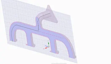
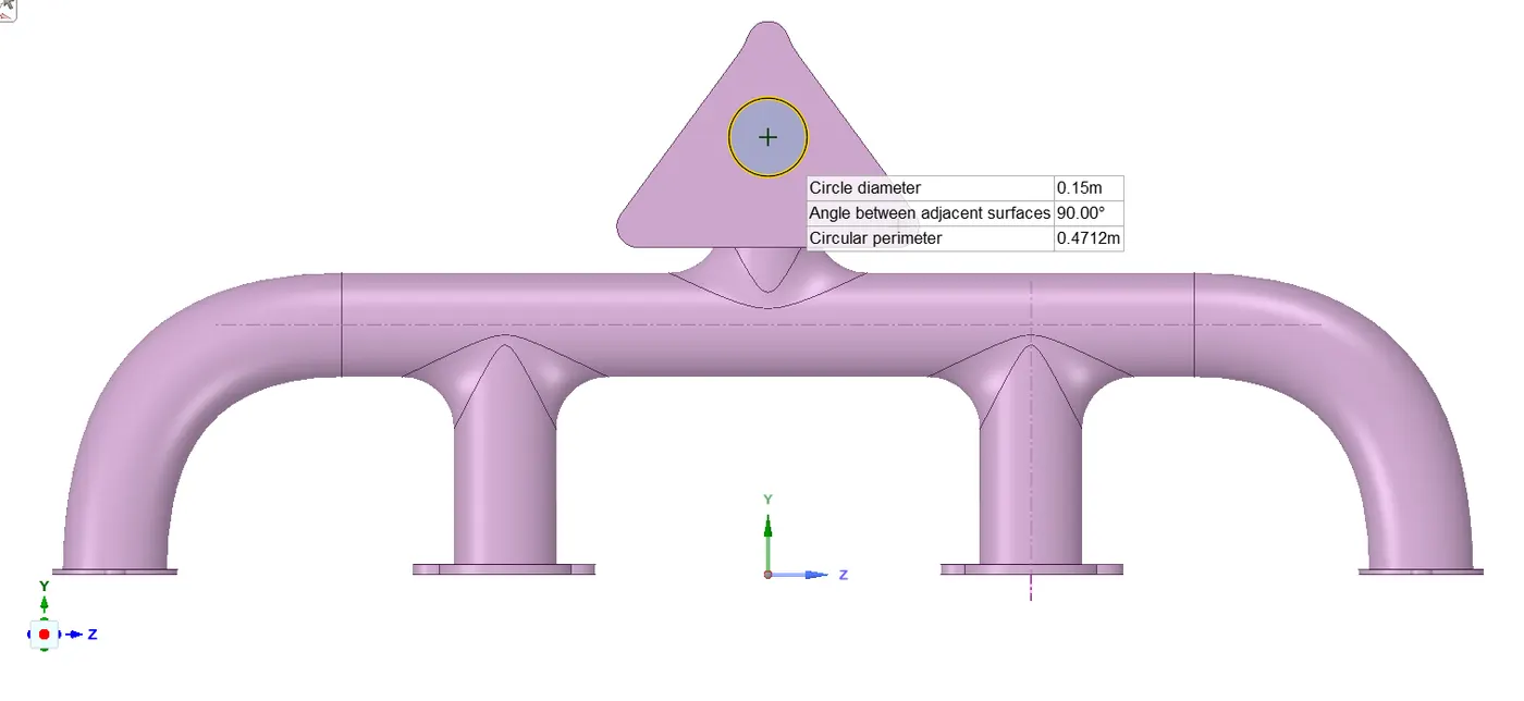
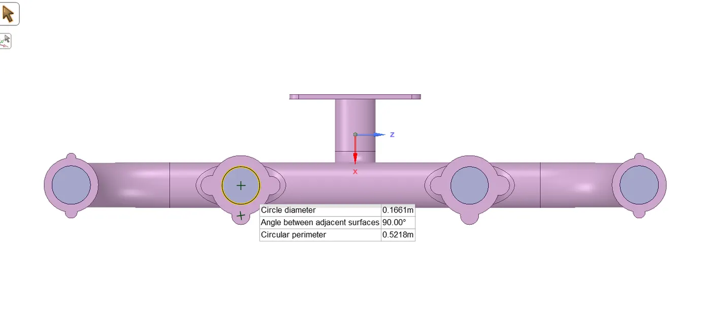
Initially, SpaceClaim is launched and the geometry which is in STEP format is imported. Fluid volume extraction is carried out. The step Workbench->Share prep takes care of creating the interfaces so that we will have only one interface between our solid and fluid volume. Once this process is done we can see a pink circle that basically tells us where the information is shared, the outer surface of the fluid volume is shared. Share topology is set to share.

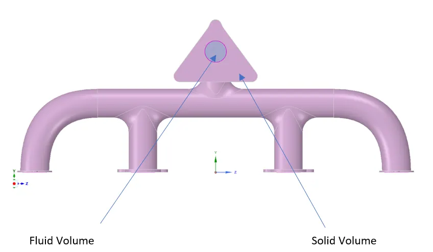
Overall Length = 2.235m

2)Meshing :

case 1 : Baseline Mesh

Mesh Element Size=100mm

Elements = 137458

Nodes = 27369

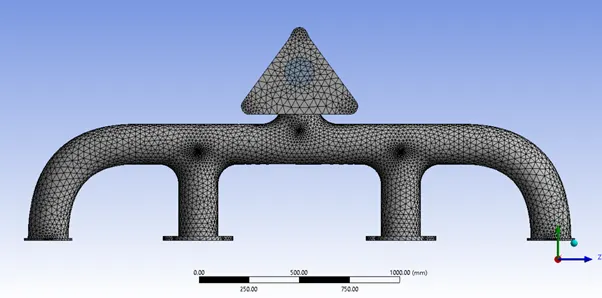
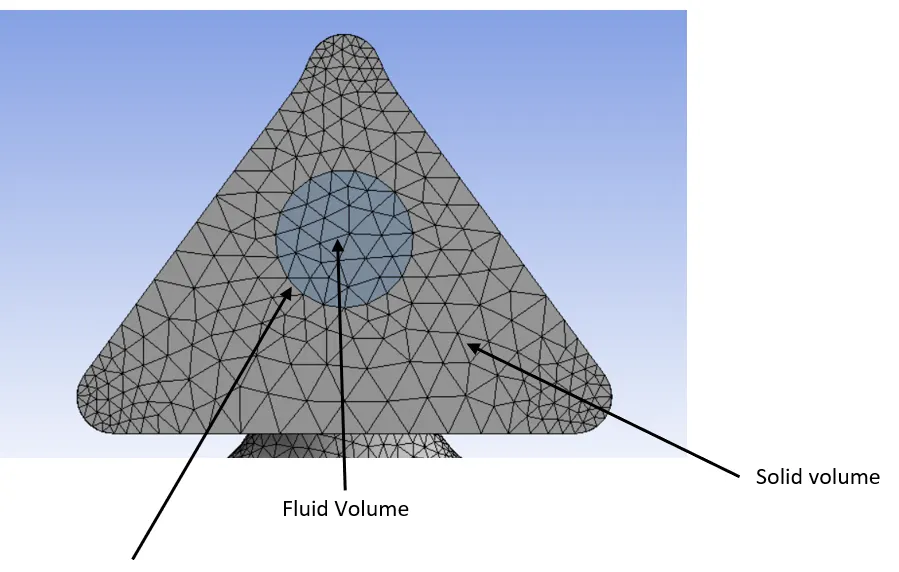
This would be the fact that both solid and fluid are going to share. The Fluid mesh will be perfectly interfacing to Solid mesh.

Named Selections :

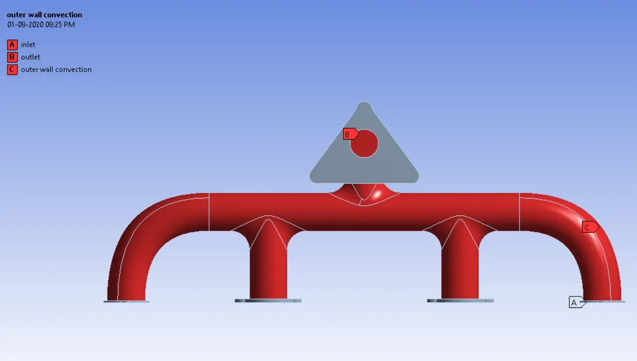
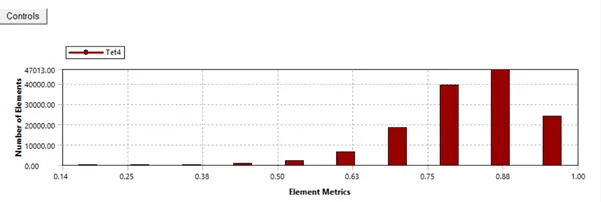
Mesh metrics: Element Quality

The mesh matric that identifies the elements according to their quality was employed, it can be seen that the mesh with low quality is minimal.

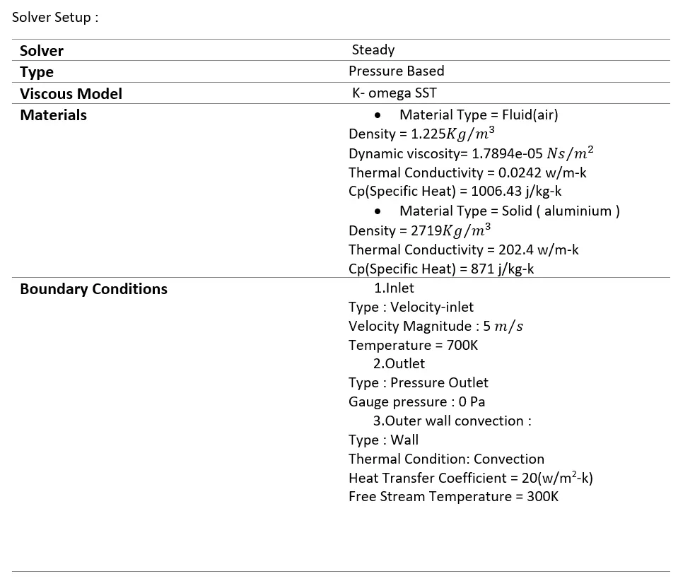
Initialize Solution: Solution is initialized from inlet region with set initial values.

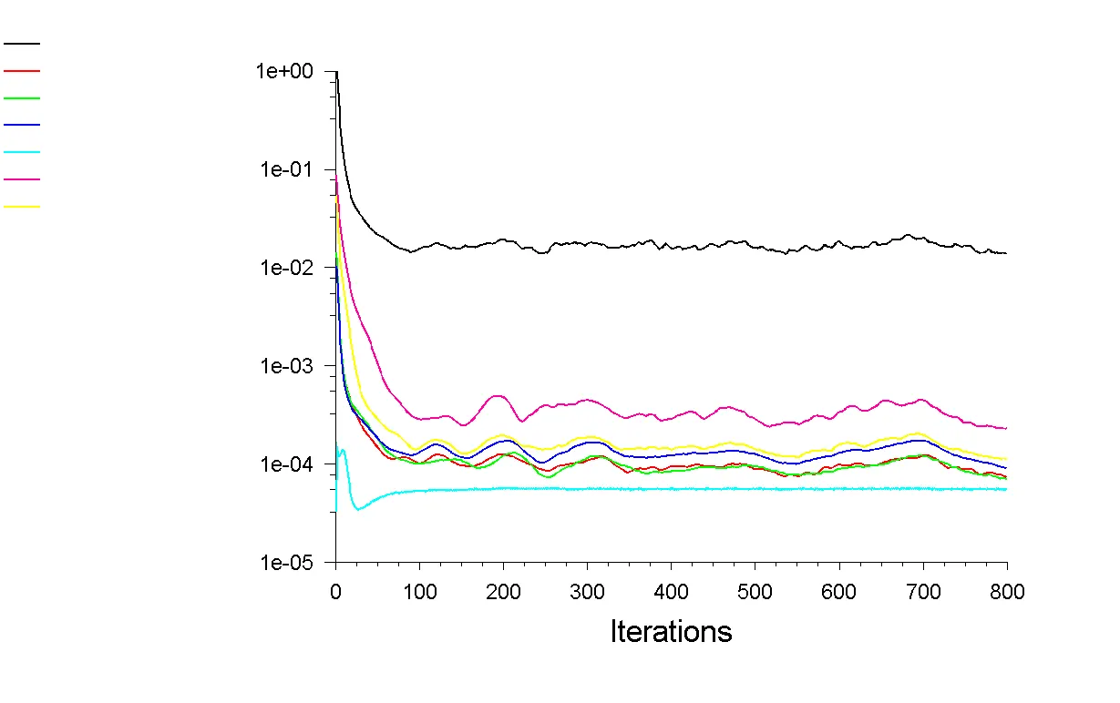
Run calculation: Number of iterations is set to 800 with a reporting interval of 1 (each iteration).

Residual Plot:

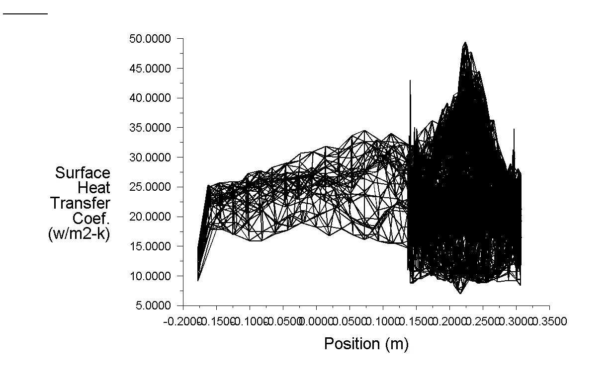
Surface HTC plot:

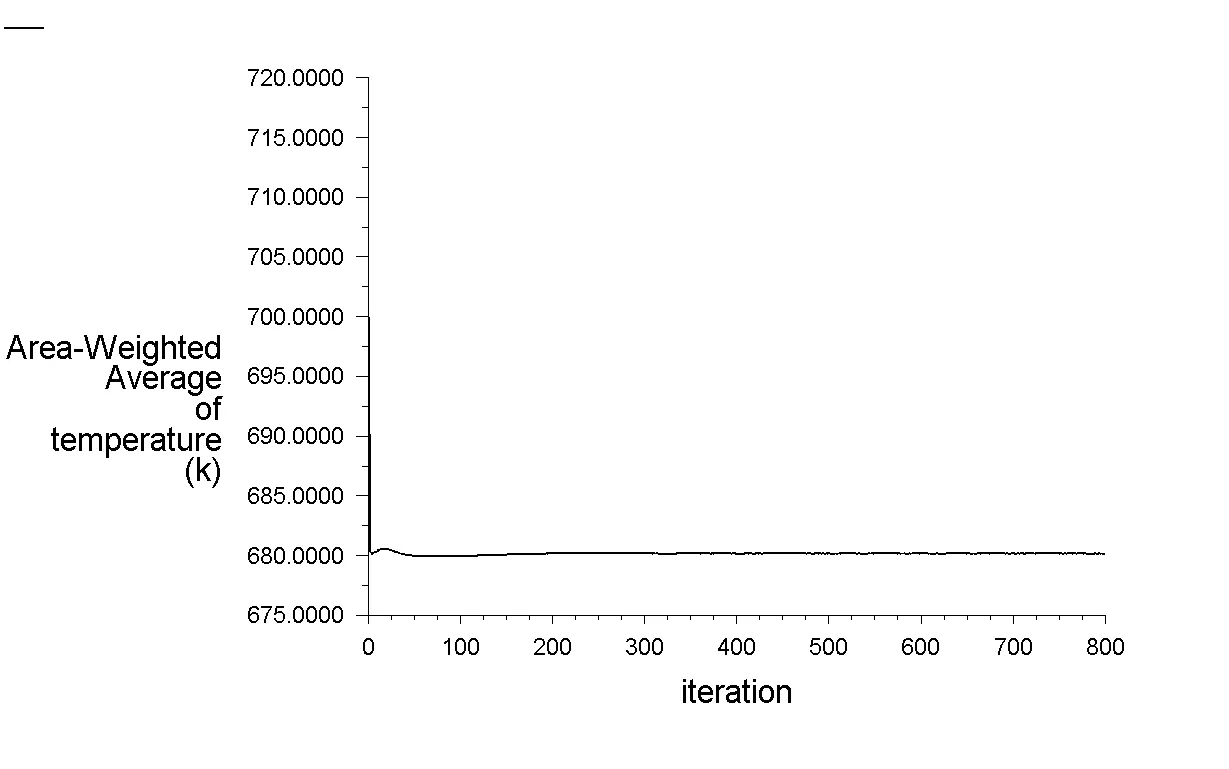
Temperature plot at Outlet :

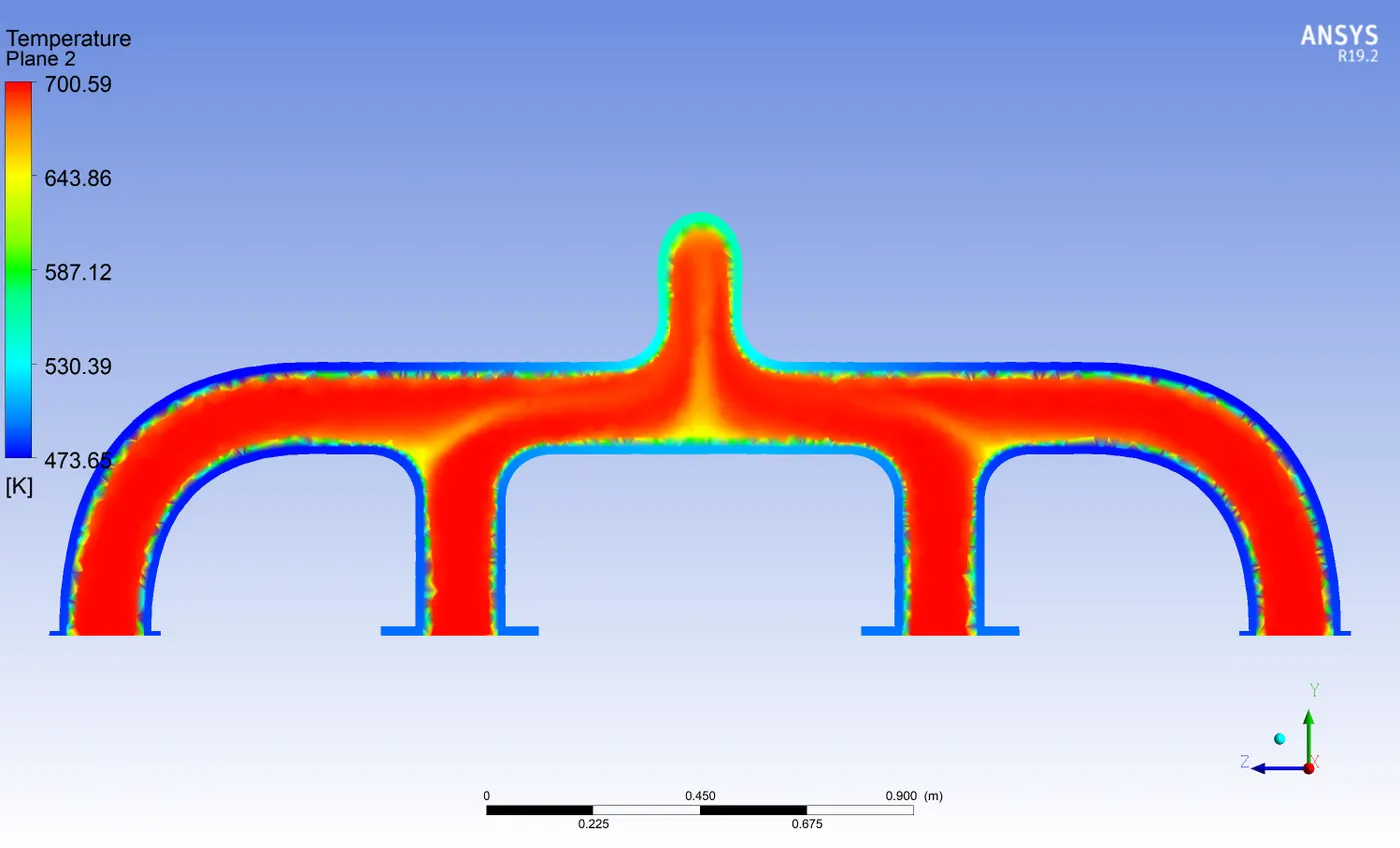
Temperature contour in Plane (a) :

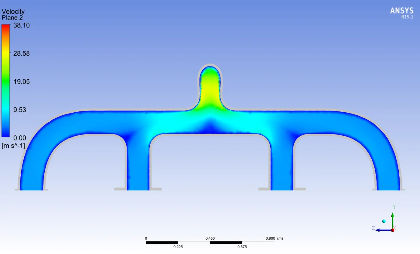
Velocity contour in Plane (a) :

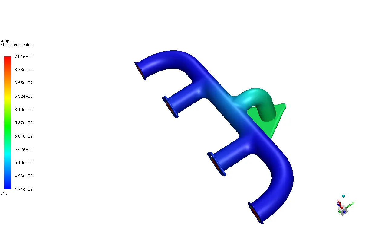
Temperature contour :

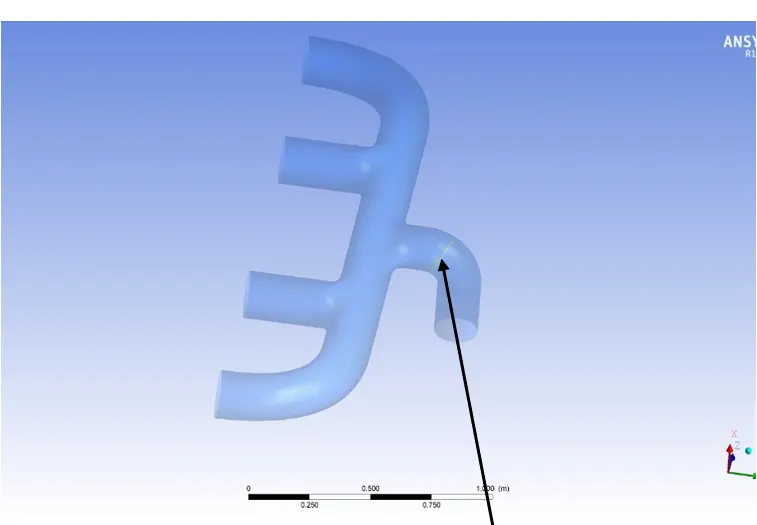
Line 1

Cut plane at the Bend :

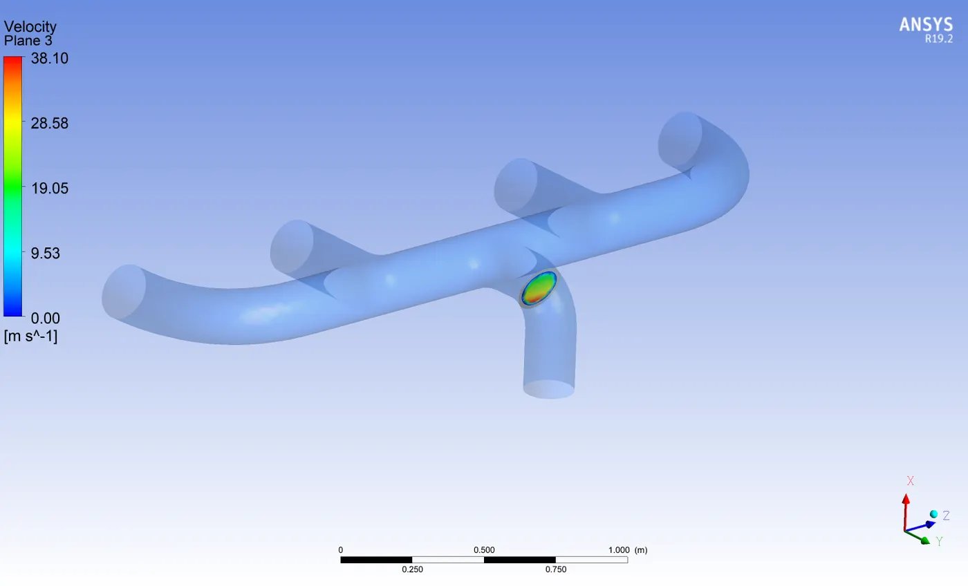
Velocity contour in a plane at outlet bend :

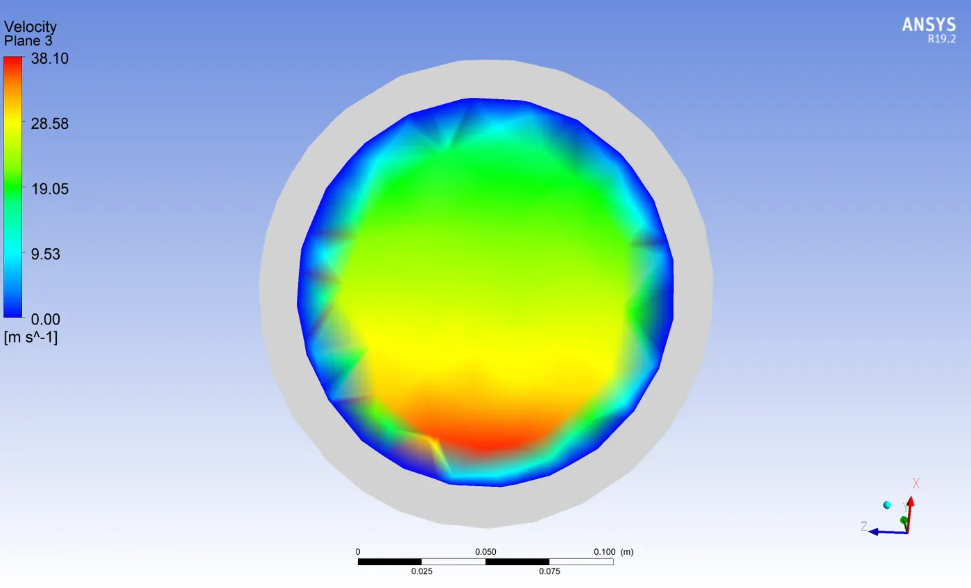
Temperature contour in a plane at outlet bend :

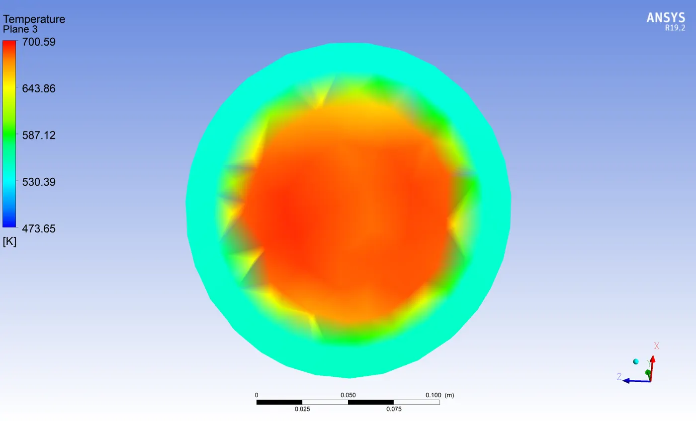
Velocity contour in a plane near the outlet :

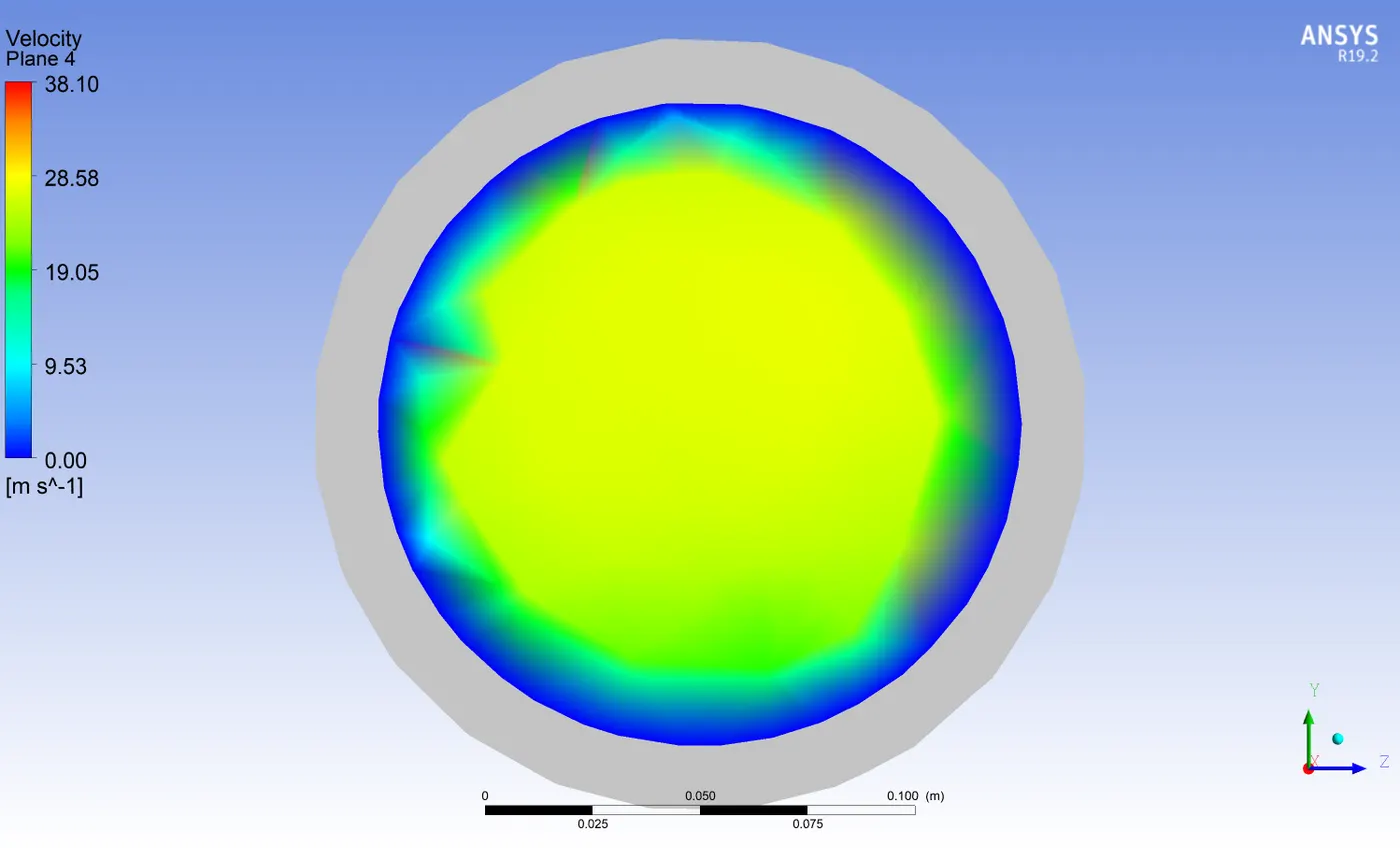
Temperature contour in a plane near the outlet :

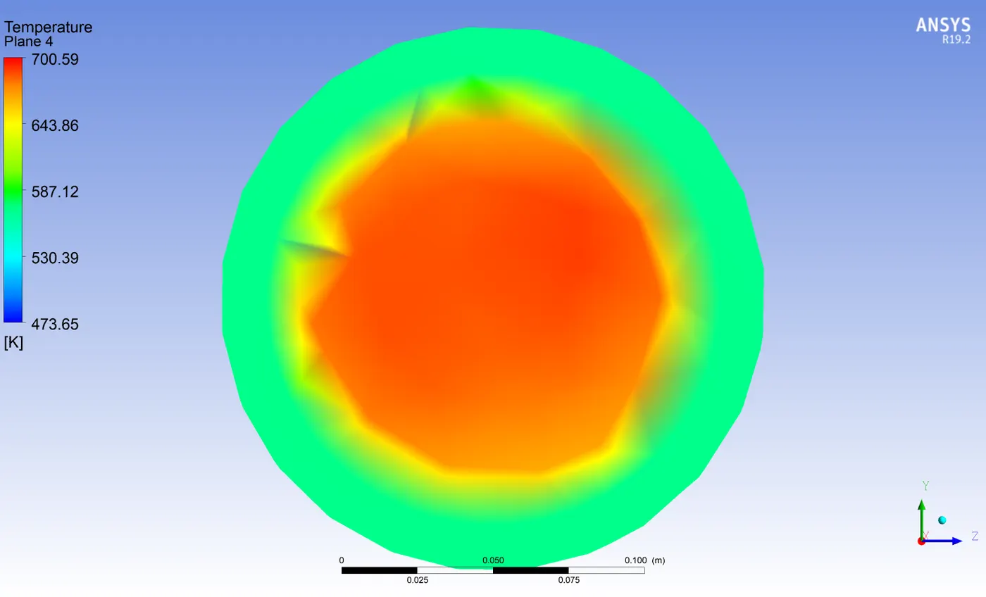
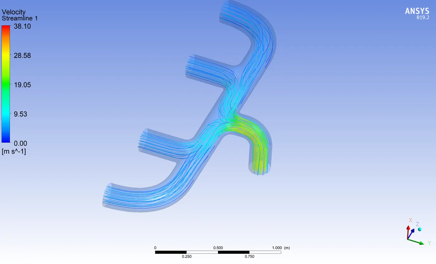
Streamlines :

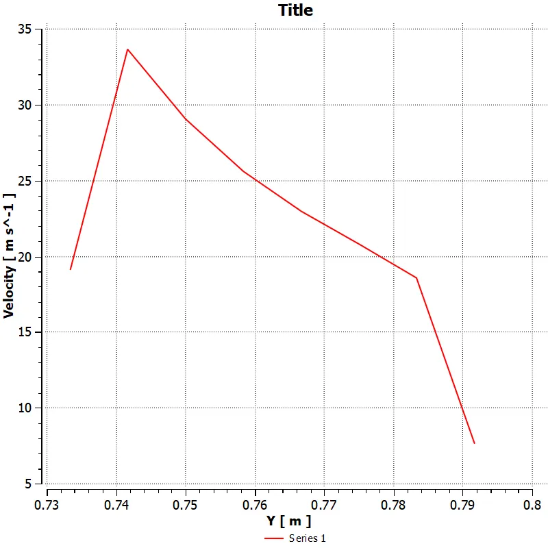
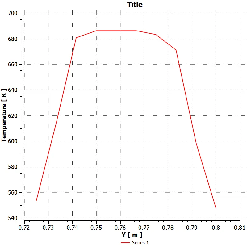
Charts :

Location: Line 1

Velocity vs Y(m) :

Temperature vs Y(m) :

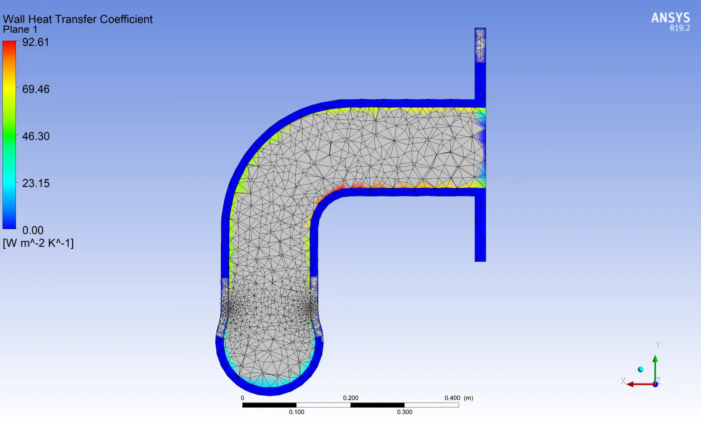
Wall HTC contour in Plane 1:

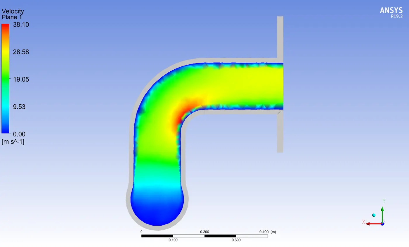
Velocity contour in Plane 1 :

Temperature contour in Plane 1 :

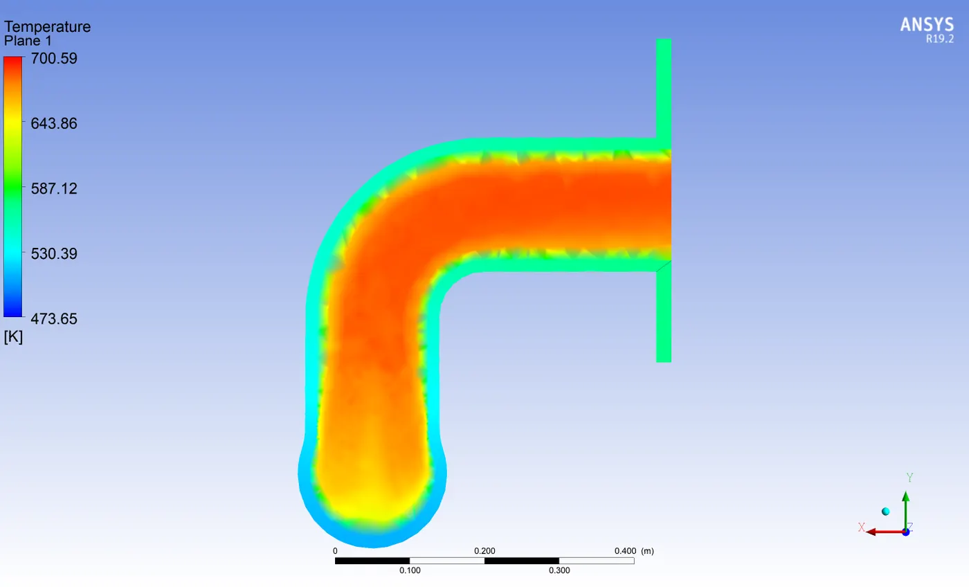
Area Weighted Average temperature at outlet = 680.2124K

Area Weighted Average Surface HTC at Inner wall = 21.3W/m²-K

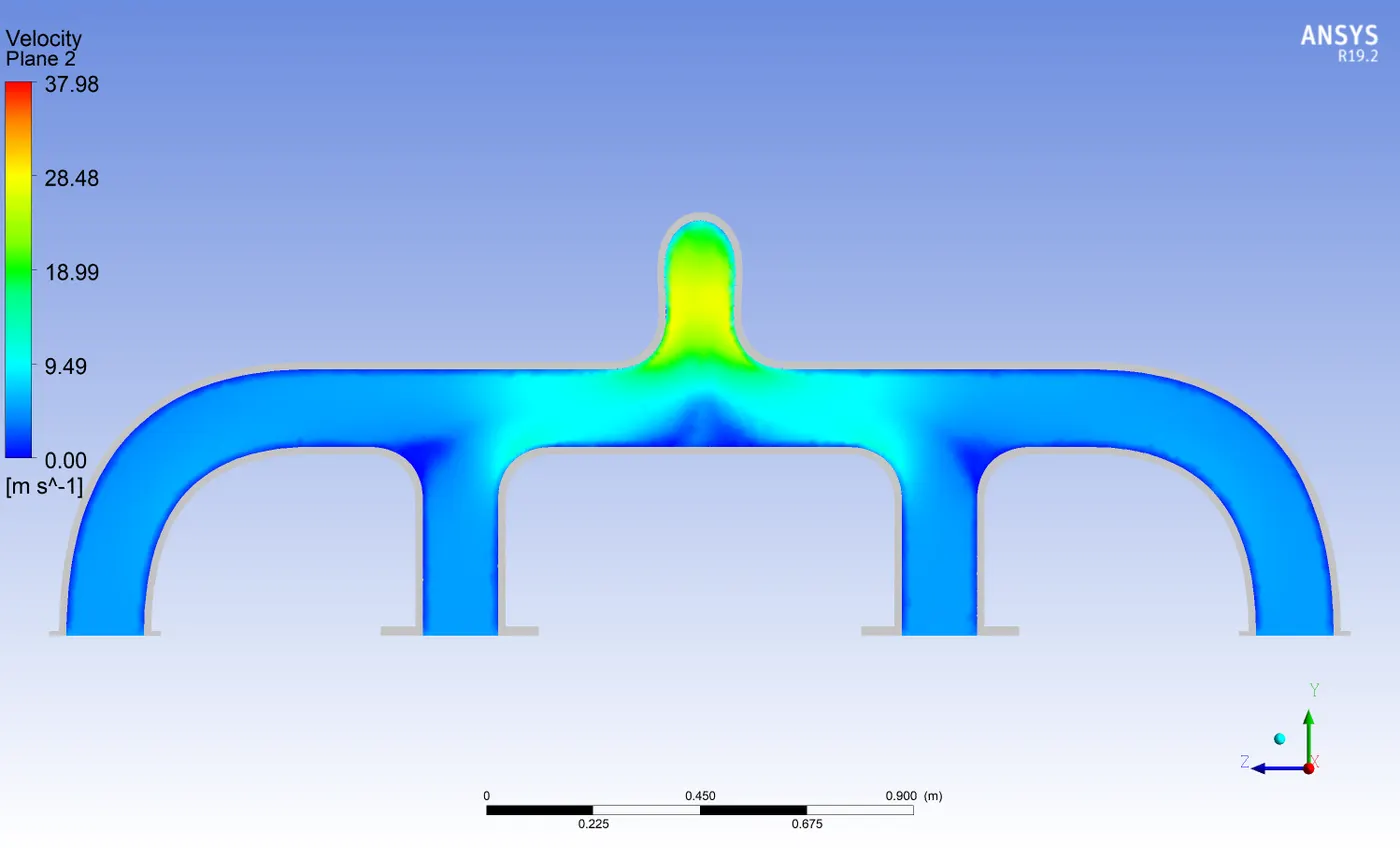
From the velocity contour shown above, it can be observed that the velocity at the bend reaches the maximum value. The exhaust port used in this project has 4 inlets and only one outlet, all the air coming through this inlet should be flown out, this makes the velocity at outlet high and results in high solid temperature. The engine is air-cooled this means it's exposed to air and the air has a particular Heat Transfer Coefficient that depends on the Reynolds number of the external air.

The velocity at the bend is high because of this Reynolds number will be high, high Reynolds number means high Heat transfer from the fluid to solid.

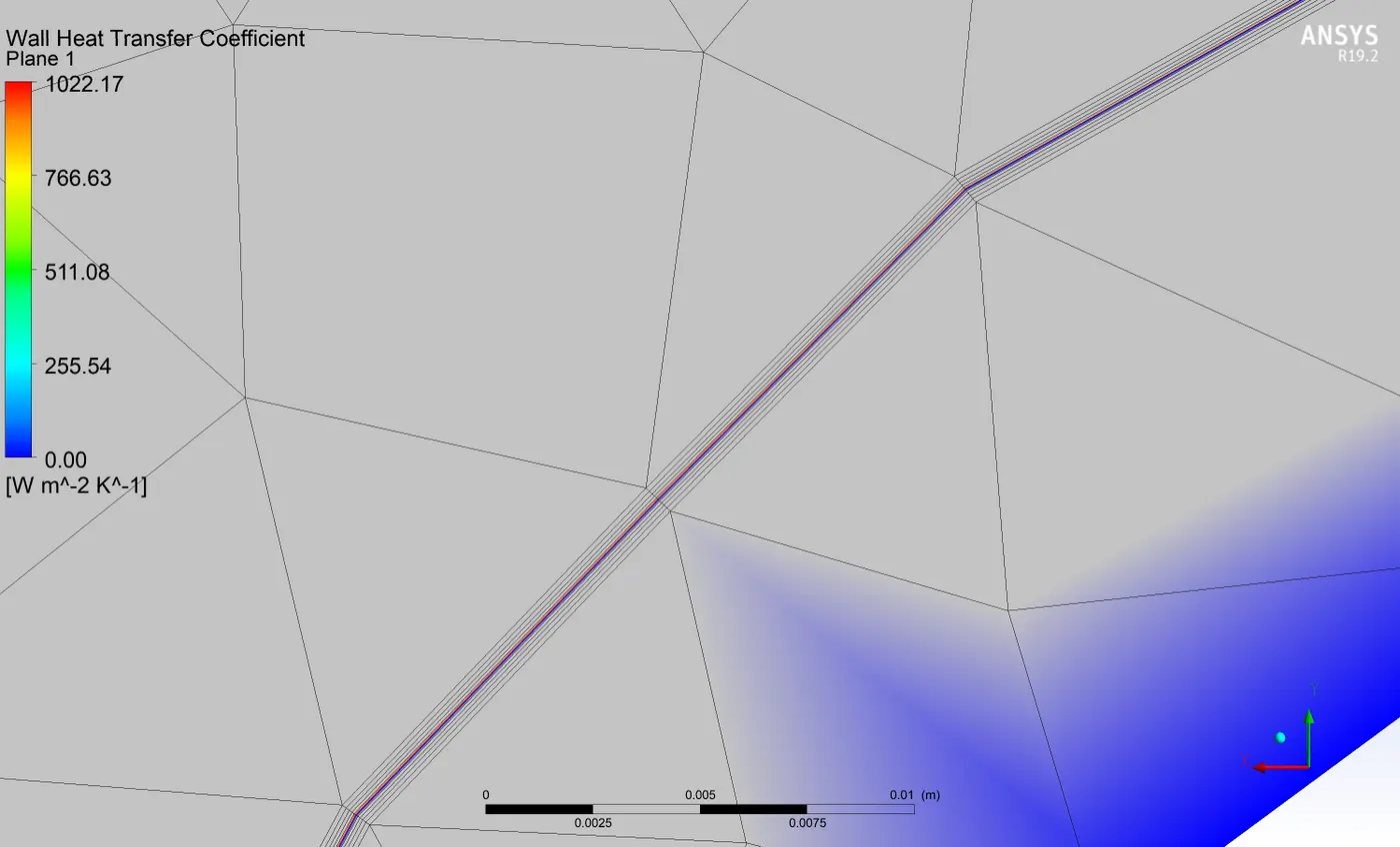
Due to the unstructured mesh near the wall we get diffused solution for heat transfer coefficient and the pattern is highly irregular. Since it’s a baseline mesh simulation, further improvements in the mesh can be done to obtain desired results.

Temperature Contour Animation :

Mesh Refinement :

Case 2:

Mesh Element Size = 20mm

Cell count = 350187

Nodes = 120243

Inflation :

Use Automatic inflation: All Faces in Chosen Named selections

Named selection: Inner wall

Inflation option: Total Thickness

Number of Layers: 5

Growth Rate: 1.2

Maximum thickness: 0.415mm

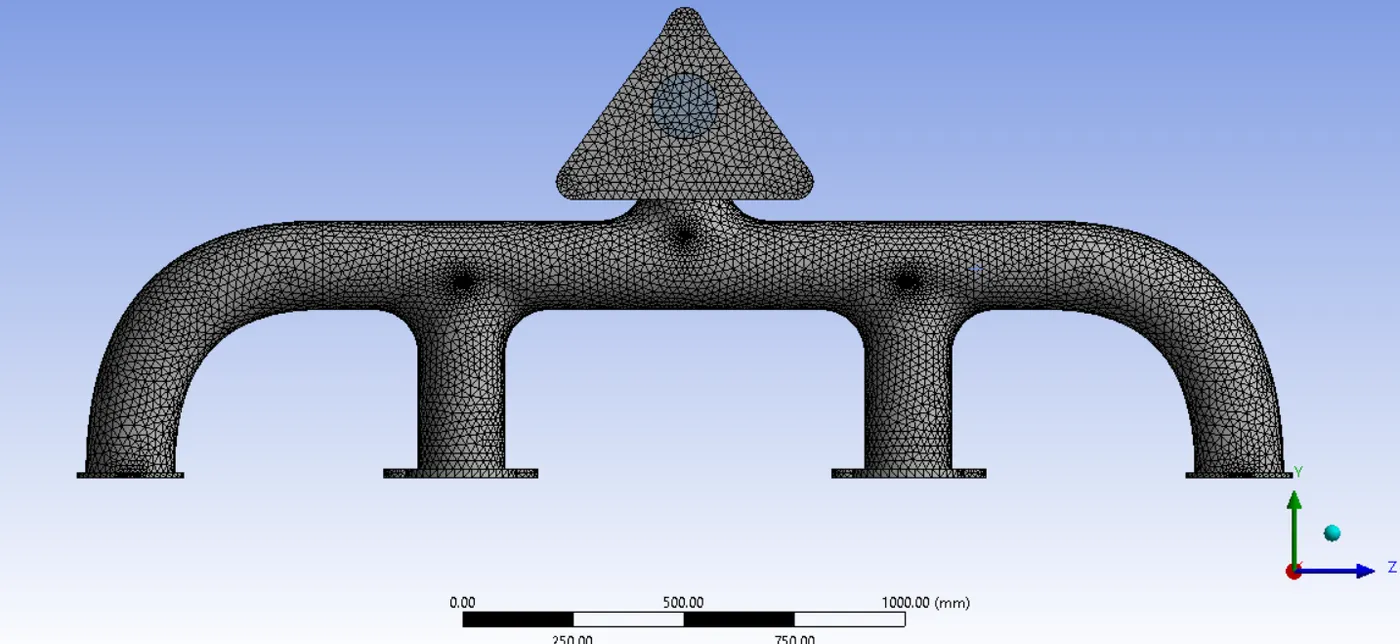
Inflation layers :

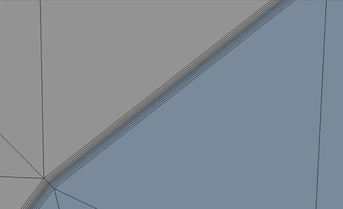
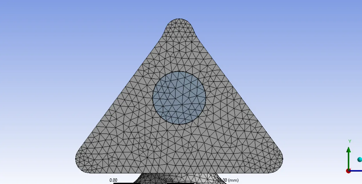
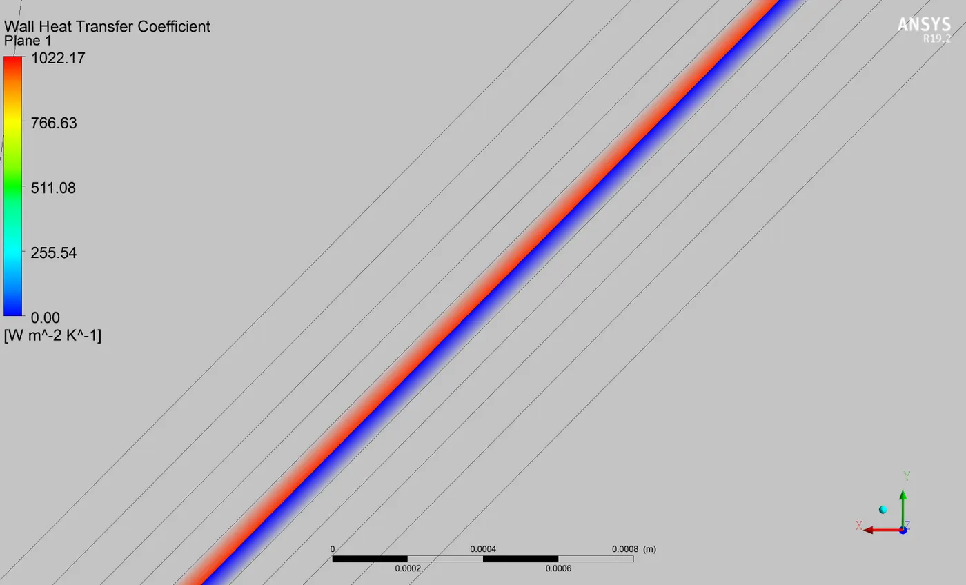
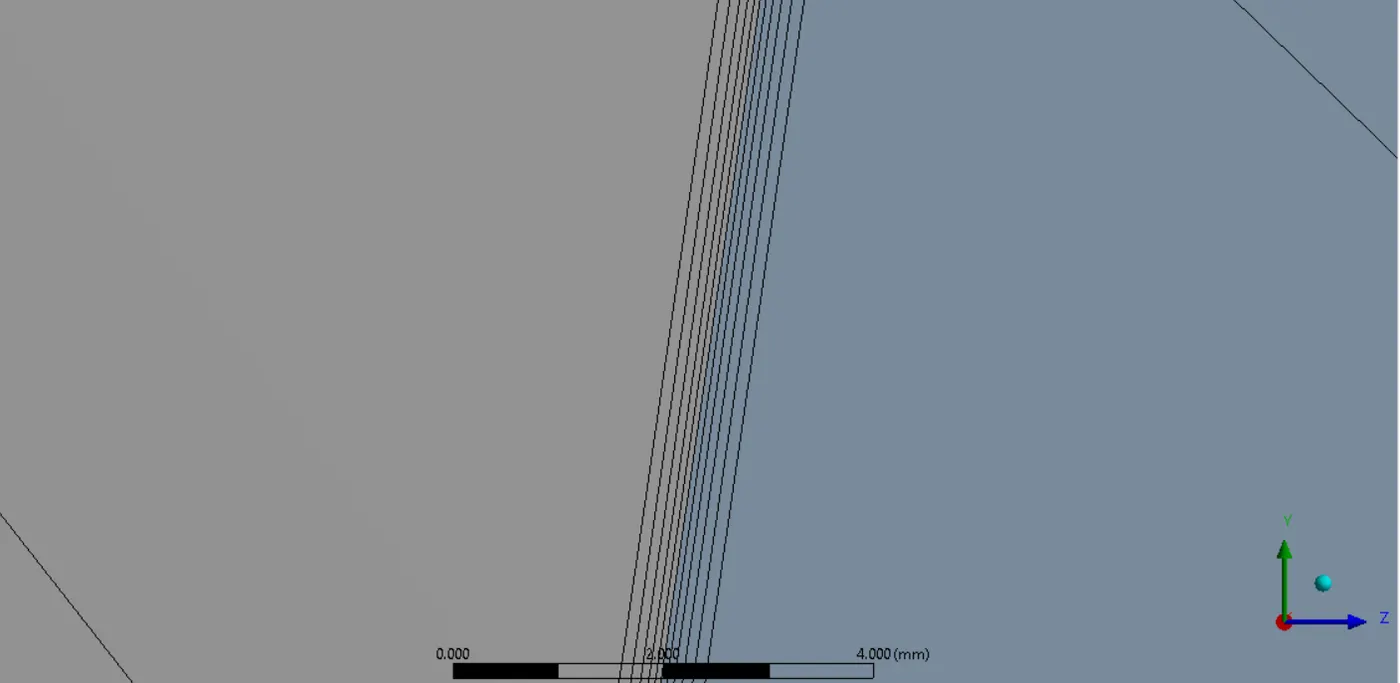
The reason for adding Inflation layer is it creates Body fitted mesh and we get smooth looking quantity near the wall.

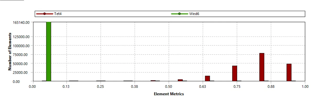
Mesh metrics: Element Quality

The mesh matric that identifies the elements according to their quality was employed, it can be seen that the mesh with low quality is minimal.

Fluent Setup will remain the same

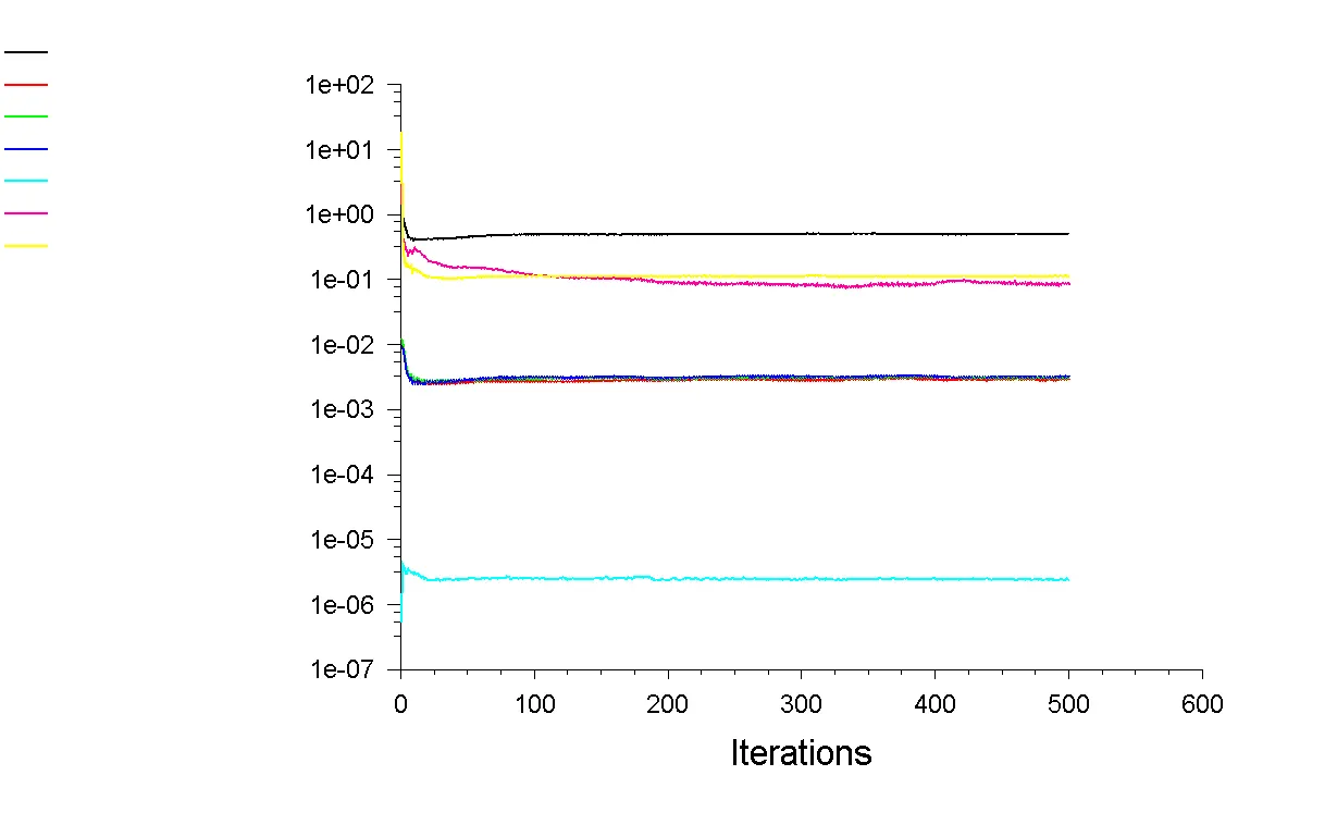
Residual Plot :

Wall HTC plot :

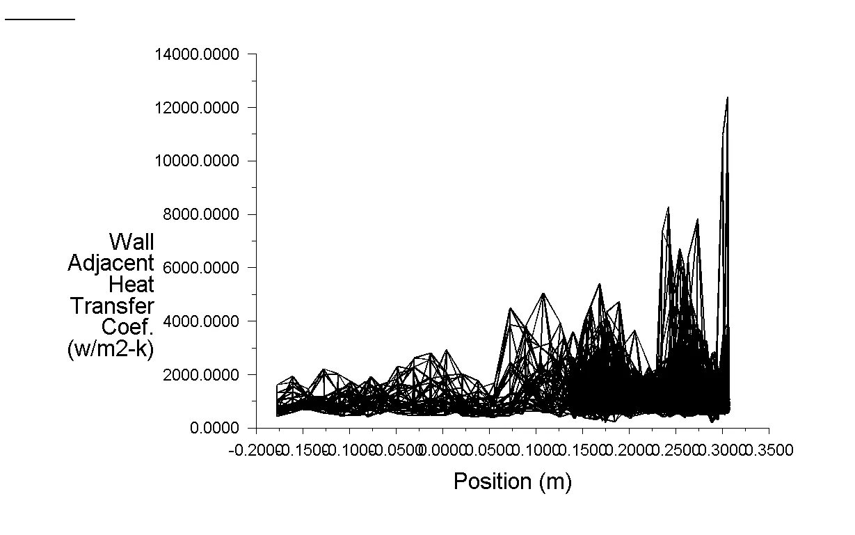
Surface HTC plot :

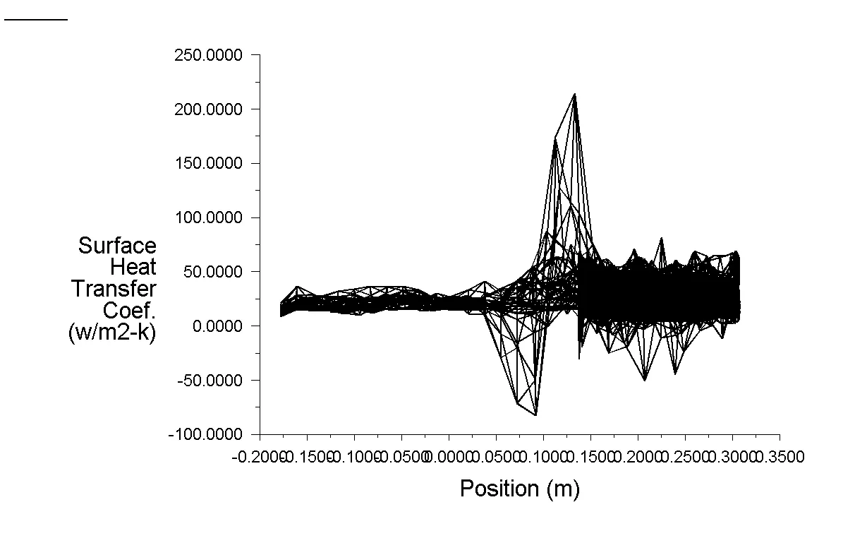
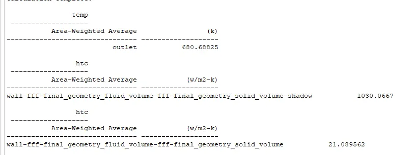
Surface HTC = 21.301 w/m^2-K

Temperature plot at Outlet :

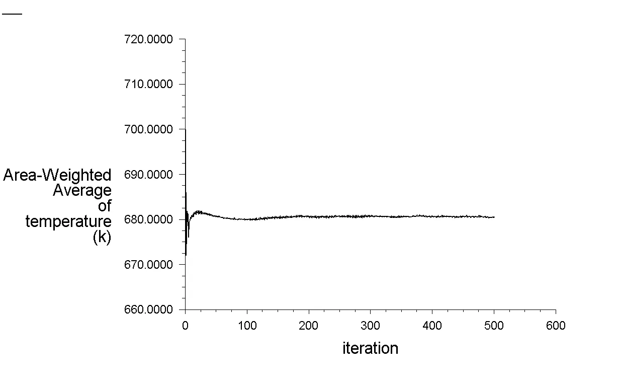
Area-Weighted Average of temperature at outlet = 680.7K

Y+ plot :

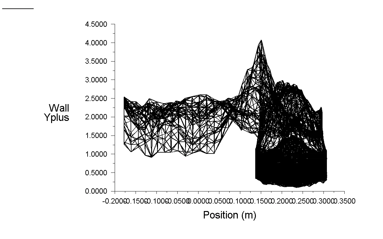
Average Y+ values are within 1 which is acceptable in this case.

Temperature contour :

Velocity contour in-plane (a):

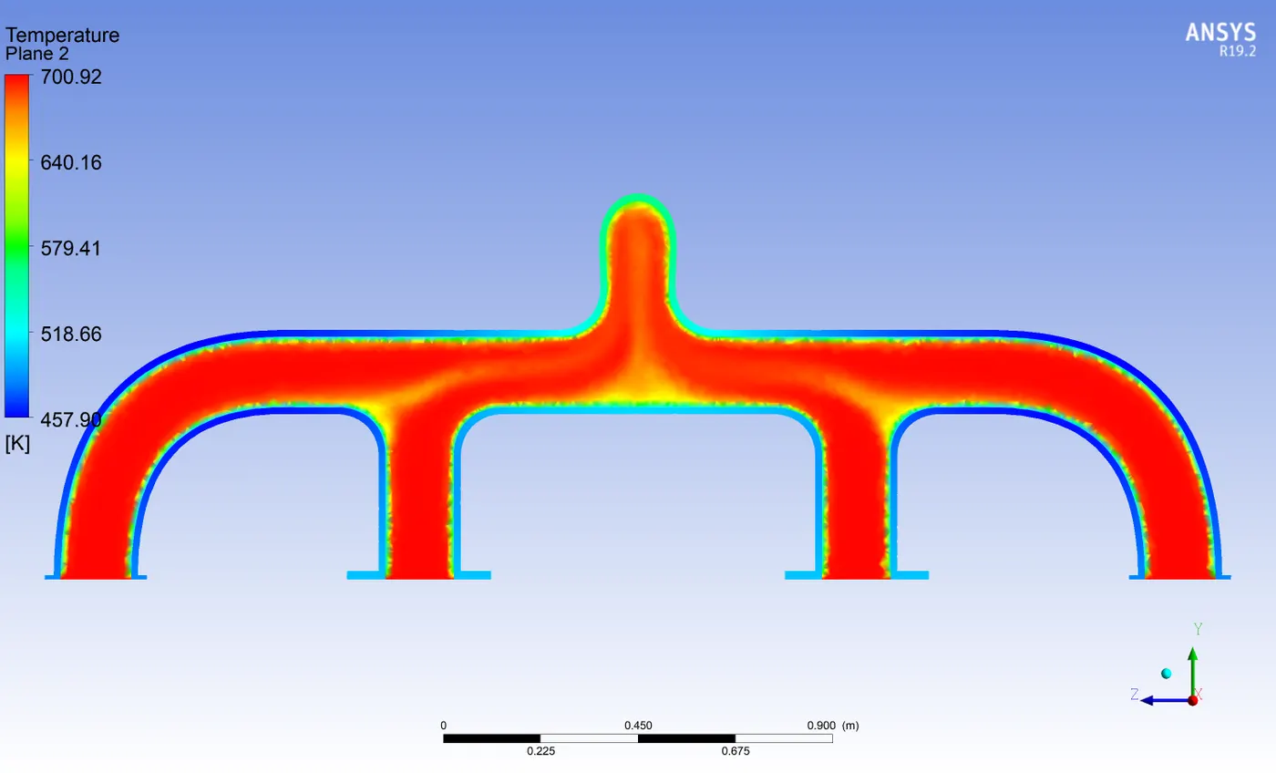
Temperature contour in Plane (a) :

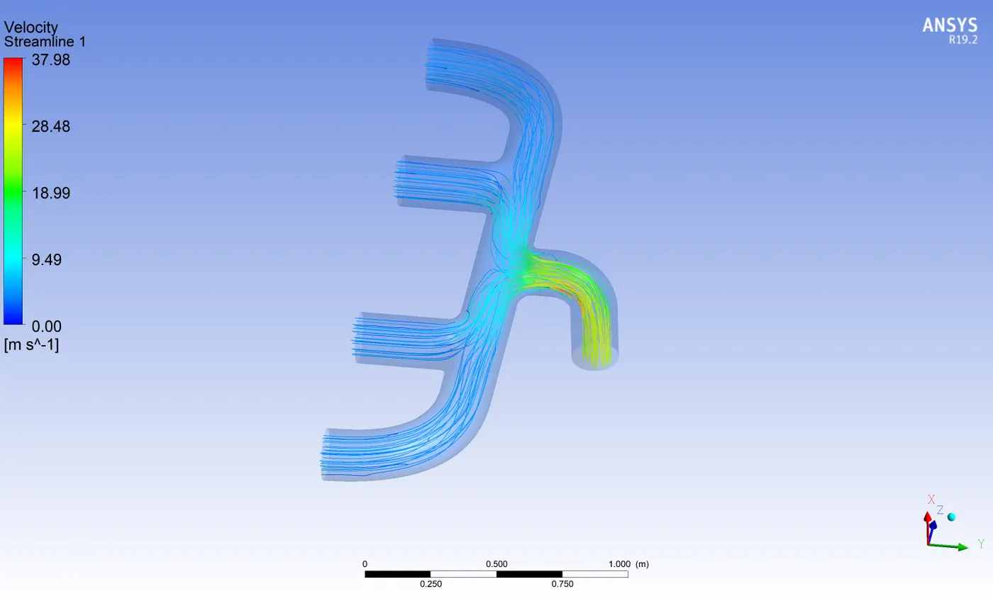
Streamlines:

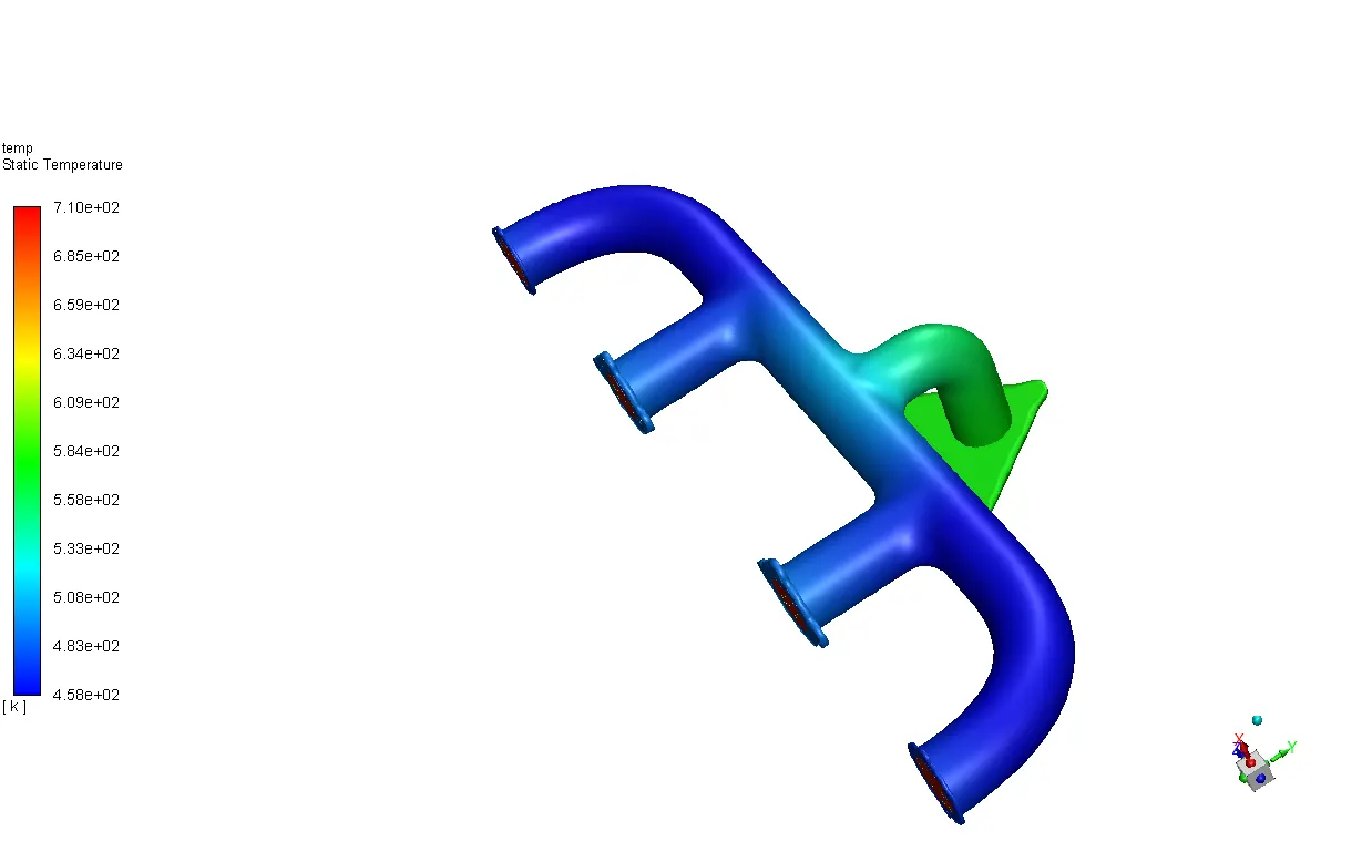
HTC contour near the wall :

Velocity contour in a plane at outlet bend :

Temperature contour in a plane at outlet bend :

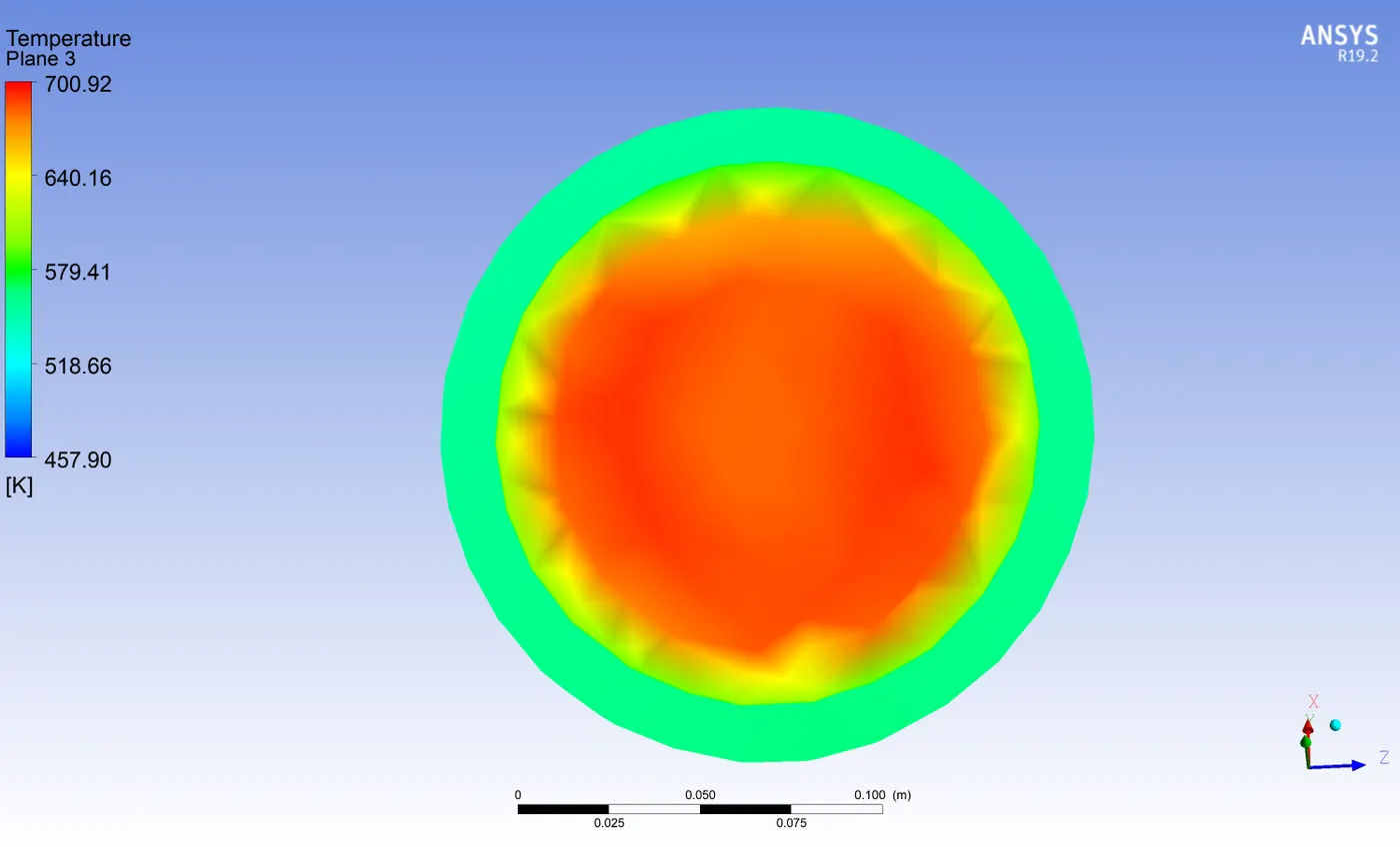
Velocity contour in a plane near outlet :

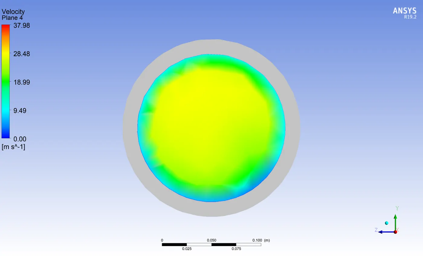
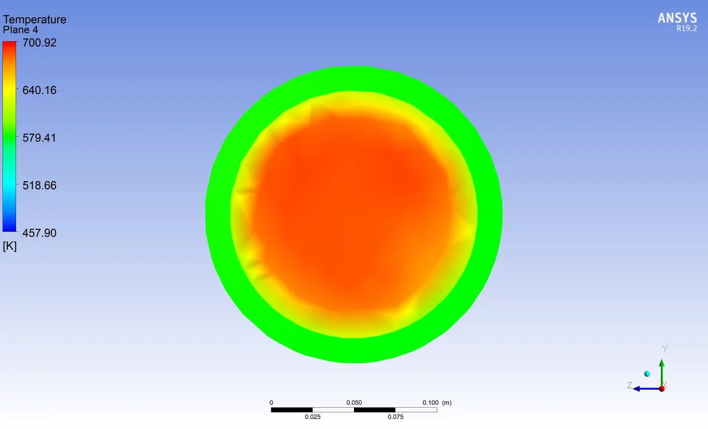
Temperature contour in a plane near the outlet :

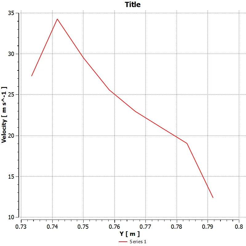
Charts:

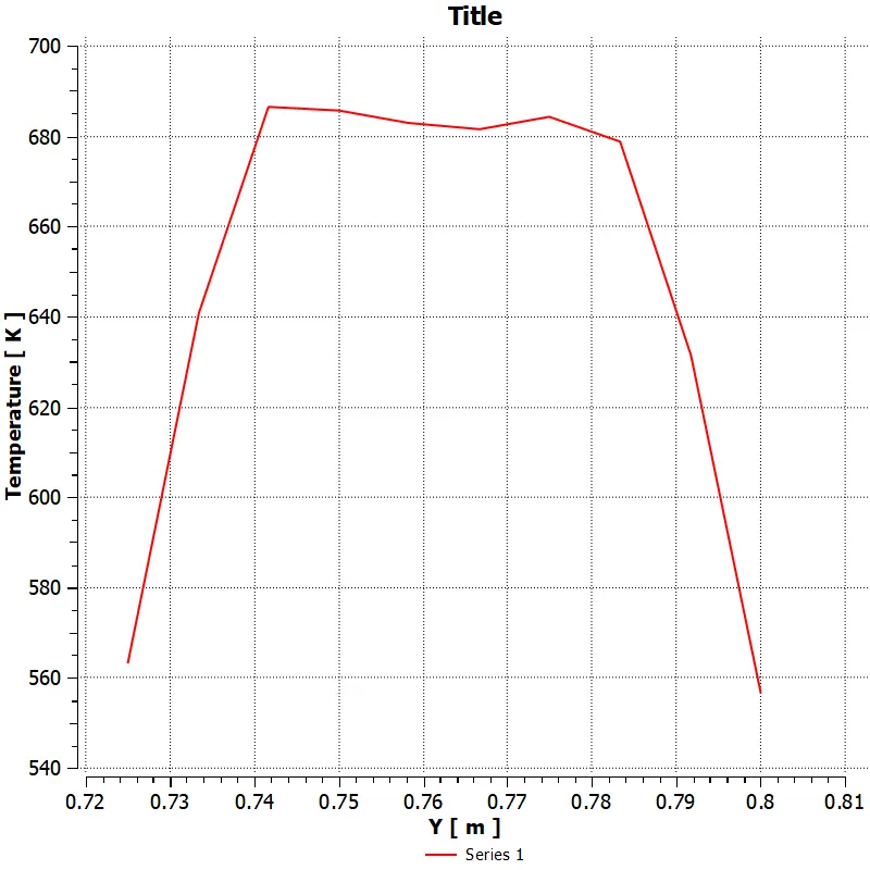
Velocity vs Y(m) :

Temperature vs Y(m) :

Velocity profile at outlet :

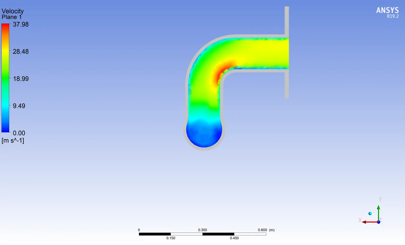
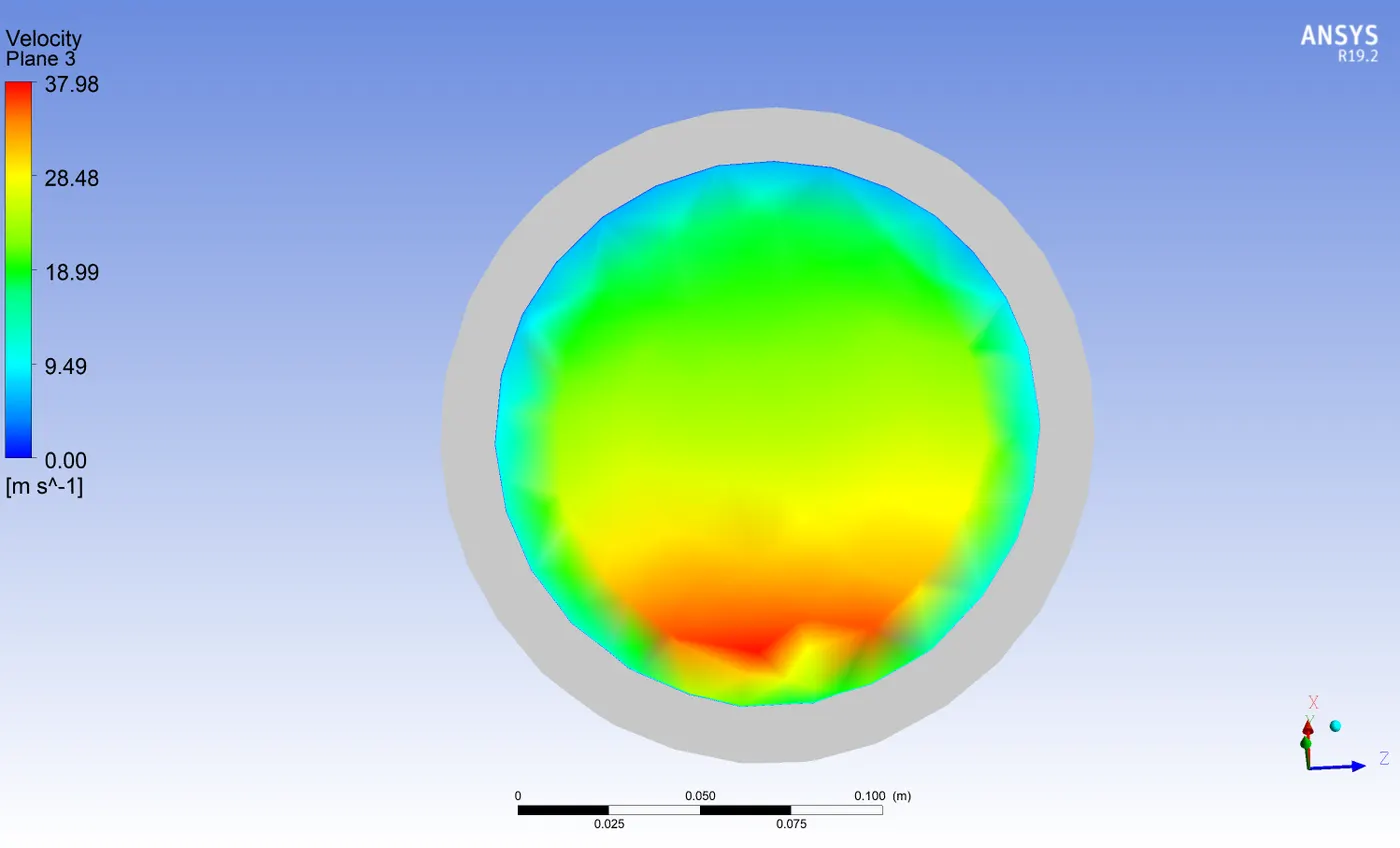
Maximum velocity on plane 1: 37.98 m/s^-1

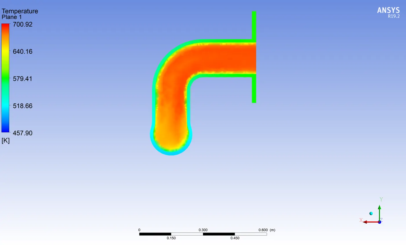
Temperature contour in Plane 1 :

Temperature Contour Animation:

Case 3 :

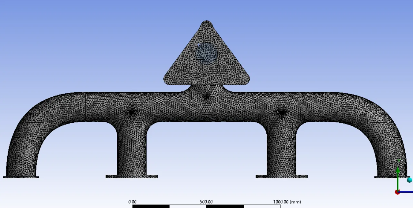
Mesh Element Size = 15mm

Cell count = 566719

Nodes = 190378

Inflation :

Use Automatic inflation: All Faces in Chosen Named selections

Named selection: Inner wall

Inflation option: Total Thickness

Number of Layers: 5

Growth Rate: 1.2

Maximum thickness: 0.415mm

Inflation Layers :

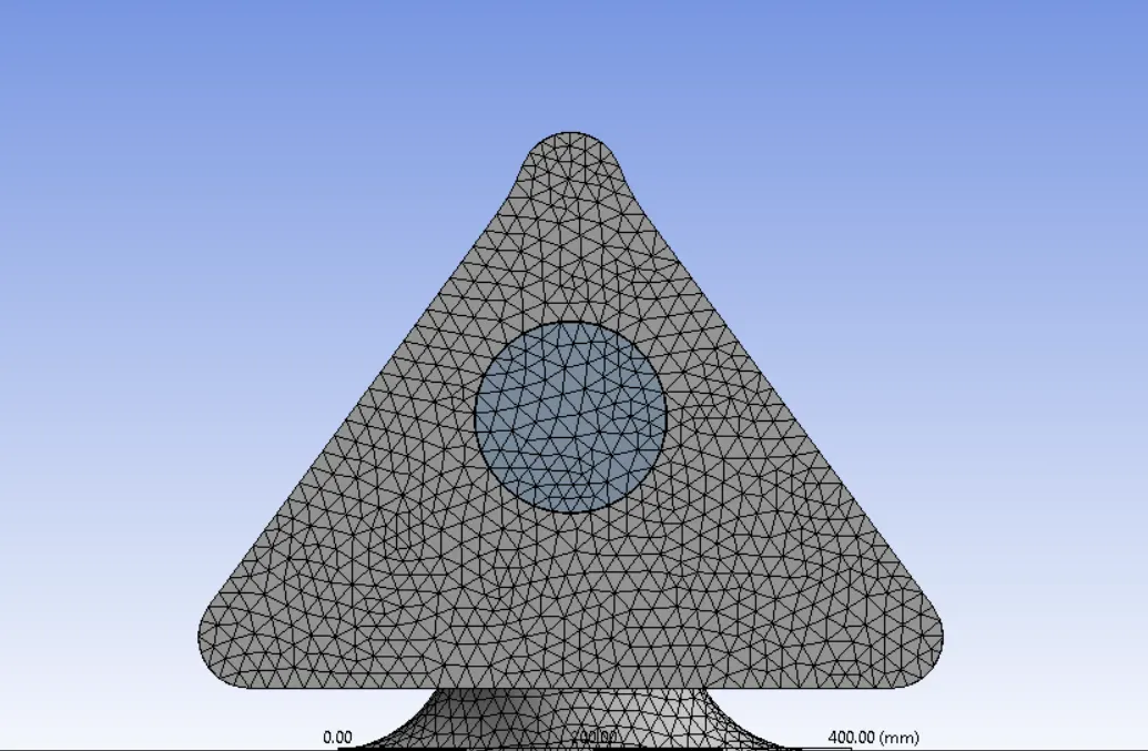
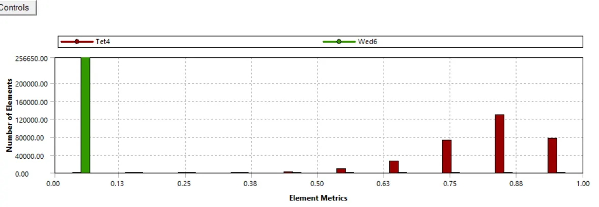
Mesh metrics: Element Quality

The mesh matric that identifies the elements according to their quality was employed, it can be seen that the mesh with low quality is minimal.

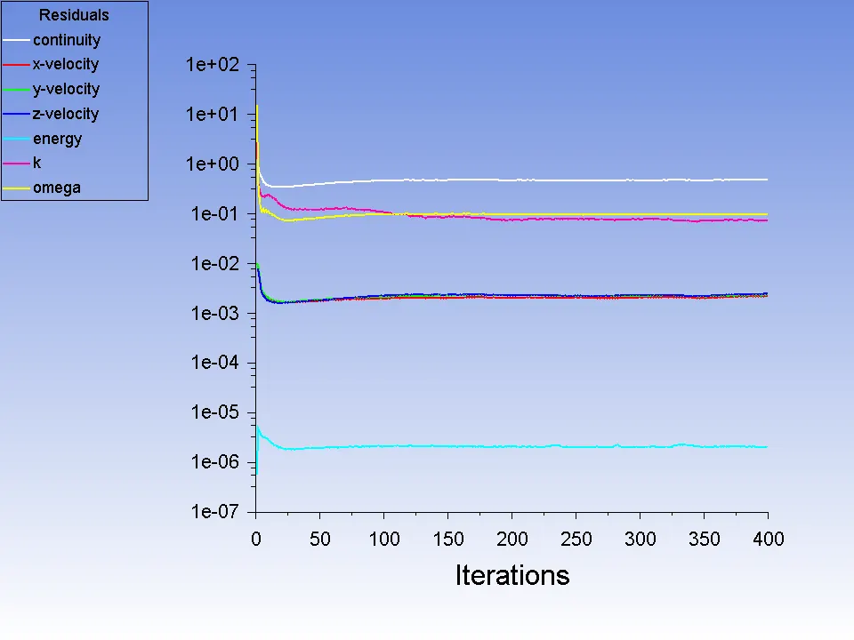
Residual Plot:

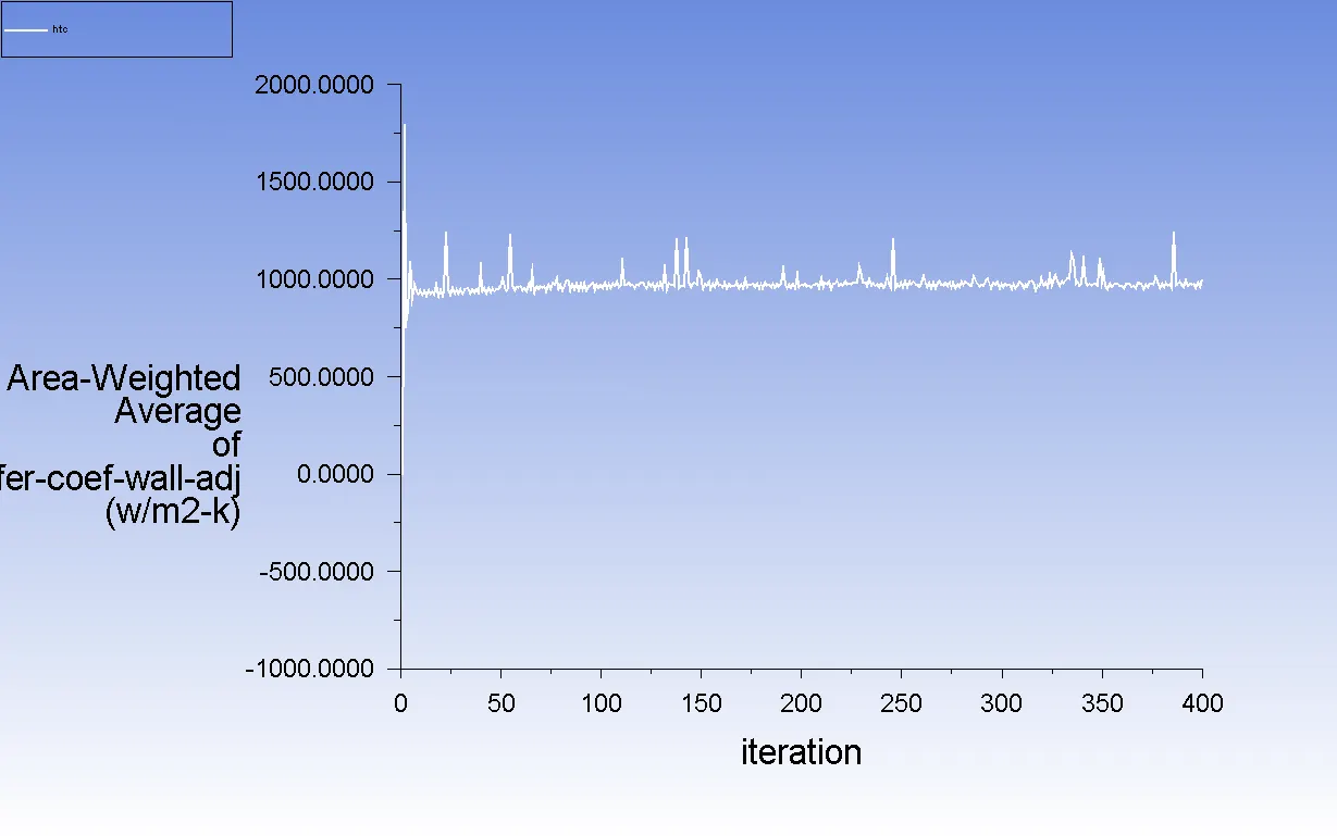
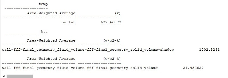
Wall HTC plot :

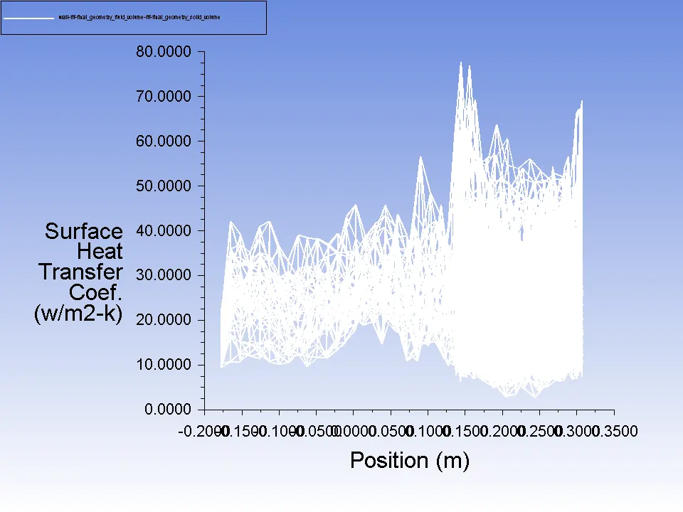
Surface HTC plot :

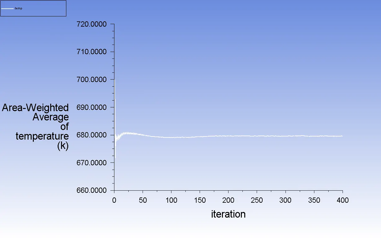
Temperature plot at Outlet :

Y+ Plot :

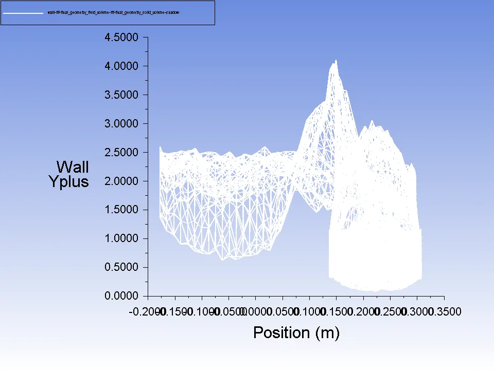
From the above Y+ plot we can say that the value of Y+ is within the acceptable limit.

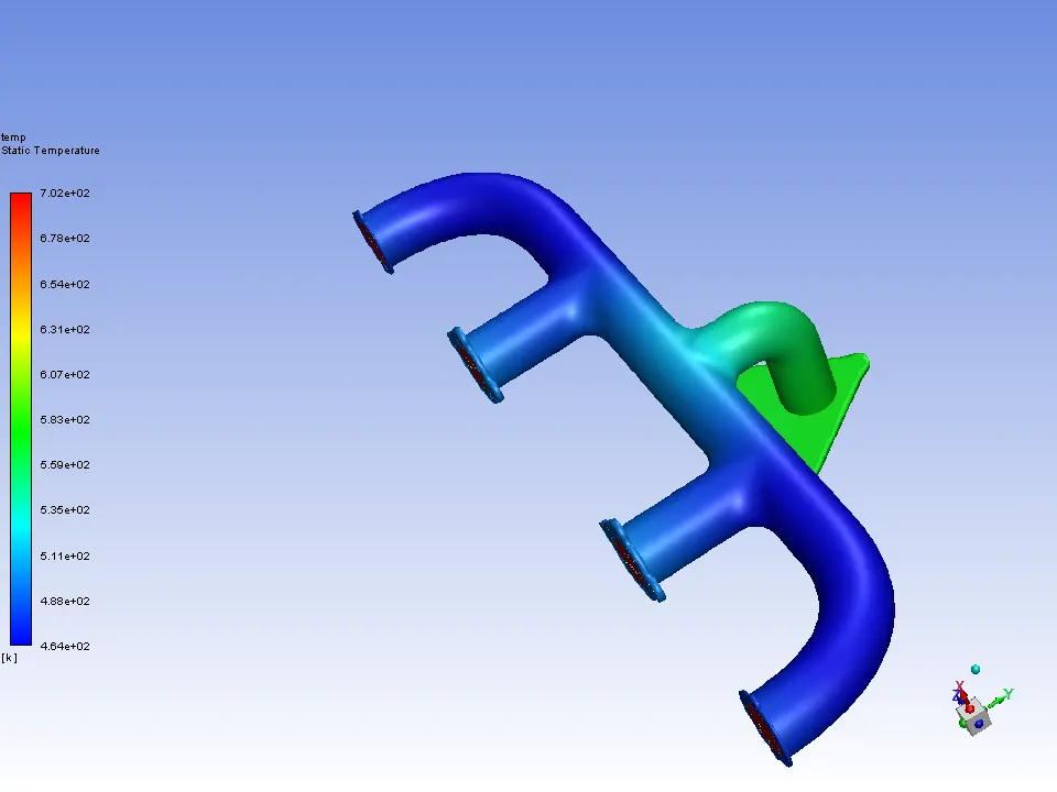
Temperature contour :

Stream Lines:

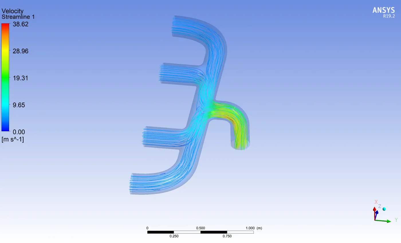
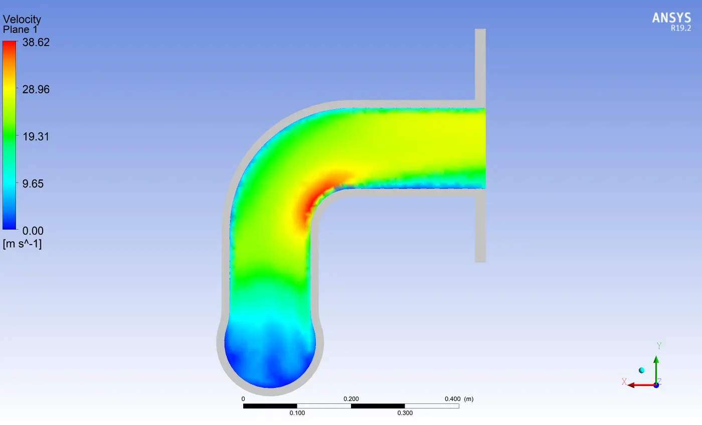
By looking at the above we can say that the velocity at the bend (outlet) reaches its maximum value of 38.62m/s^2.

Velocity contour in-plane (a) :

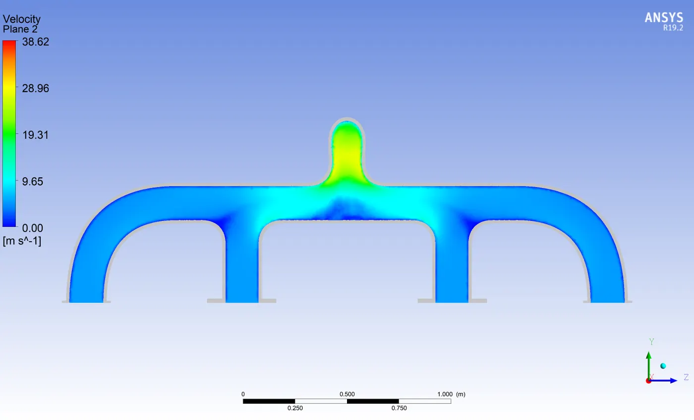
Temperature contour in-plane (a) :

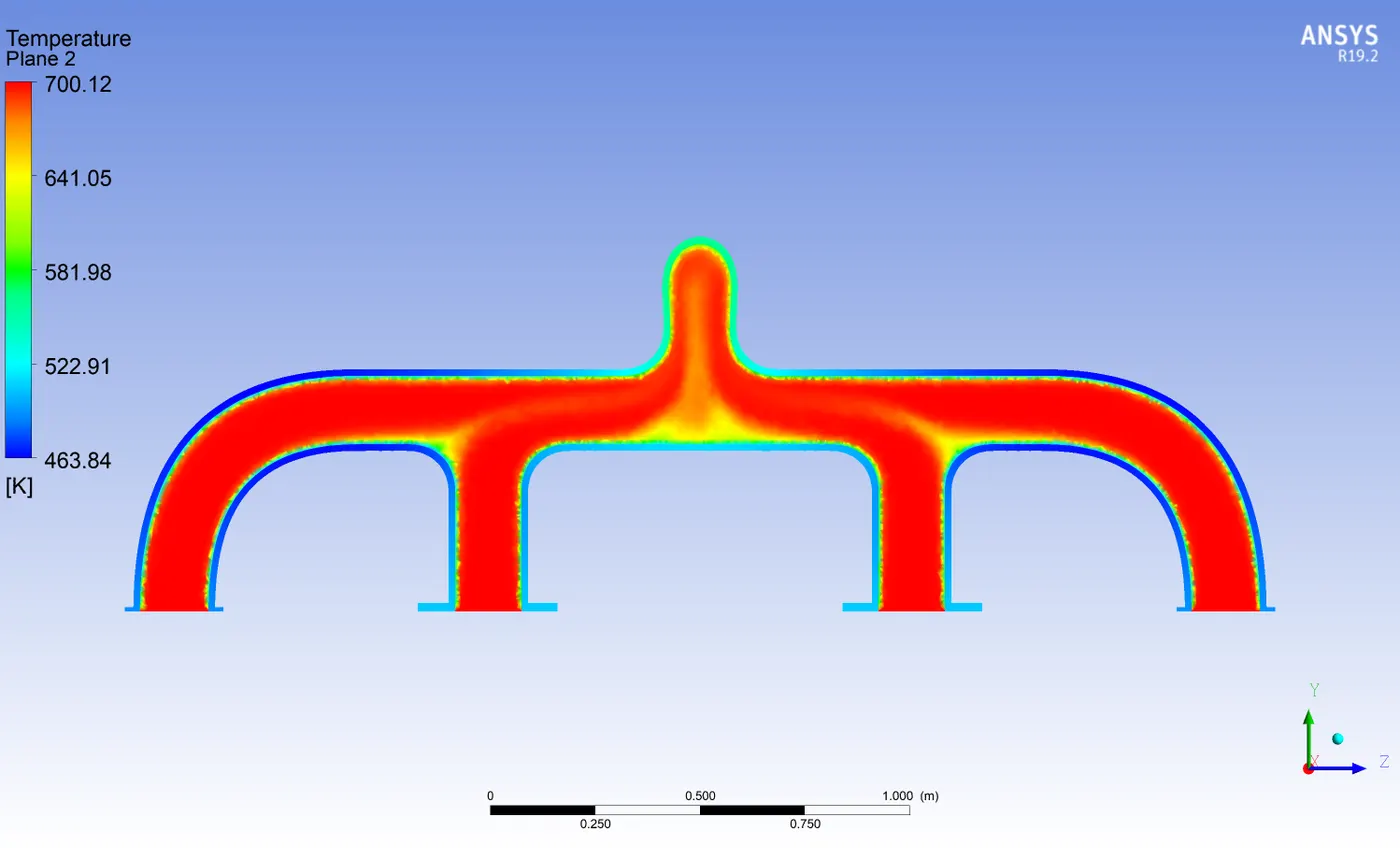
HTC contour near the wall :

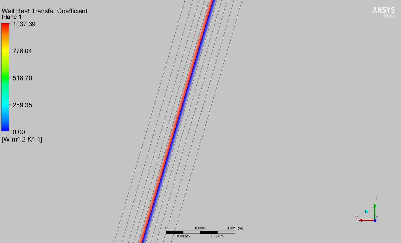
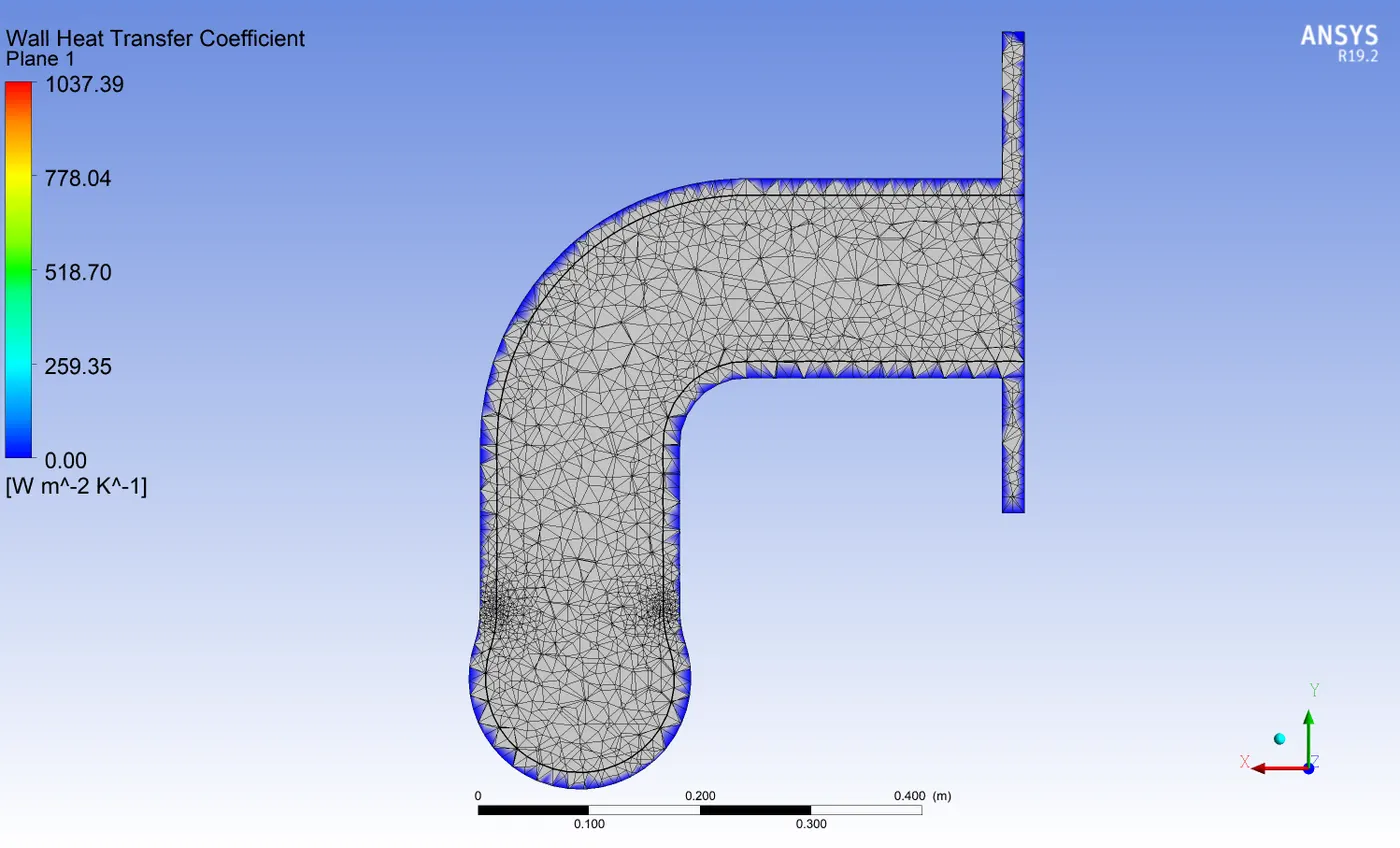
Cut Plane at the Bend :

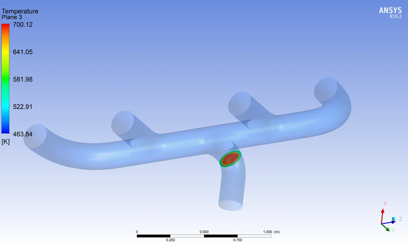
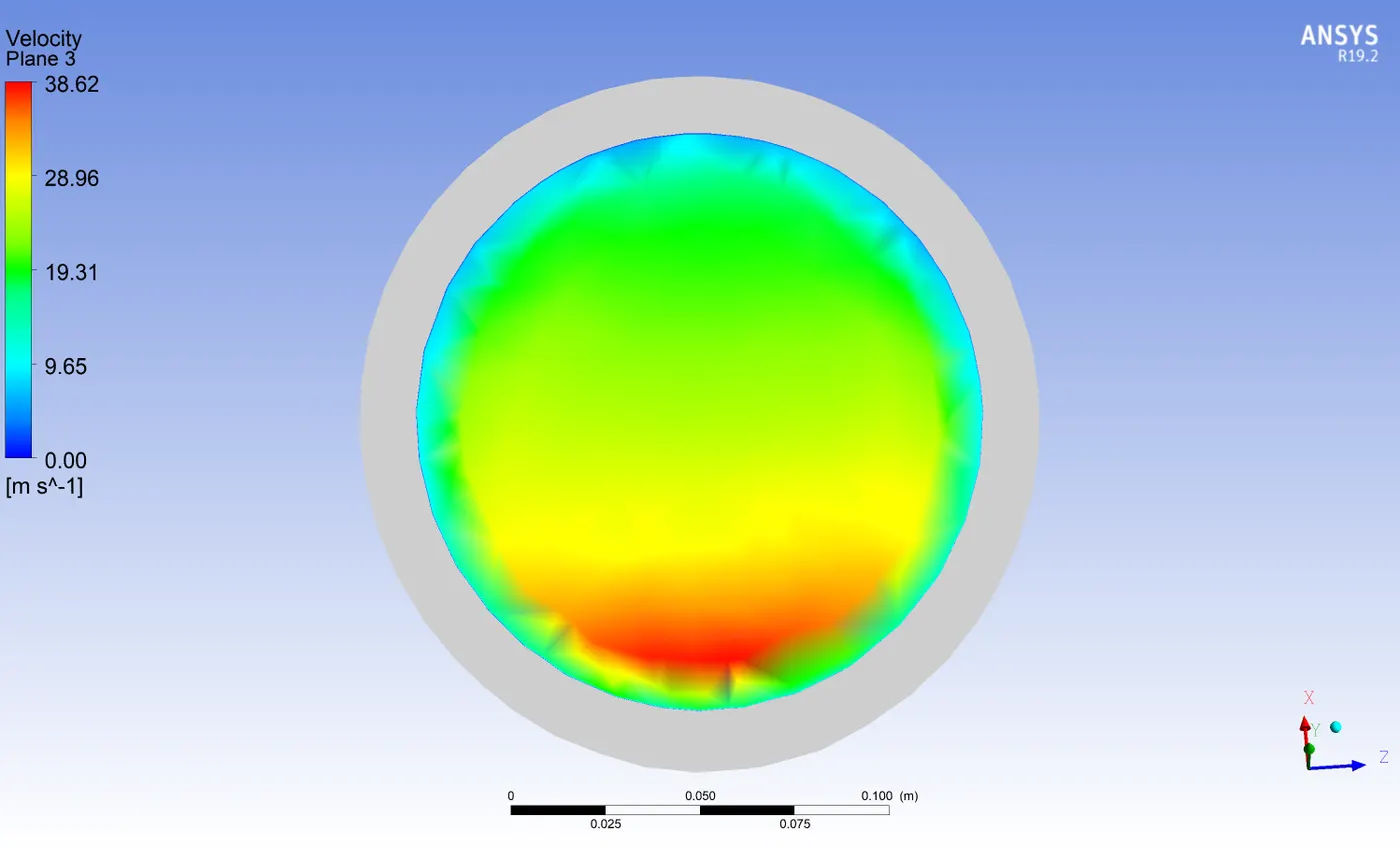
Velocity contour in a plane at outlet bend :

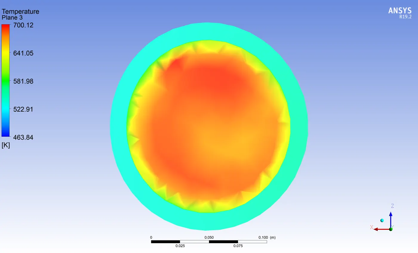
Temperature contour in a plane at outlet bend :

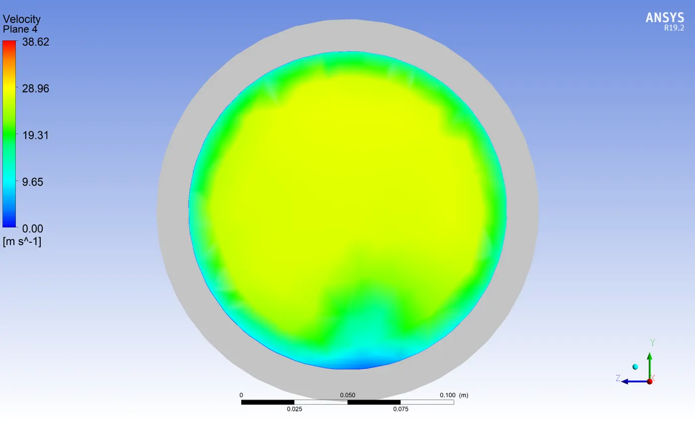
Velocity contour in a plane near the outlet :

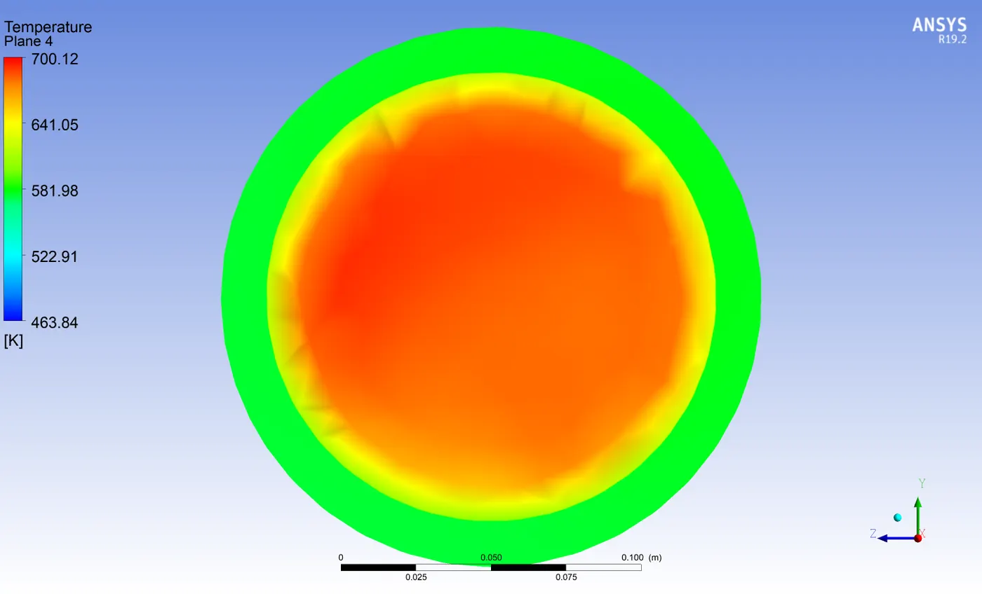
Temperature contour in a plane near the outlet :

Charts:

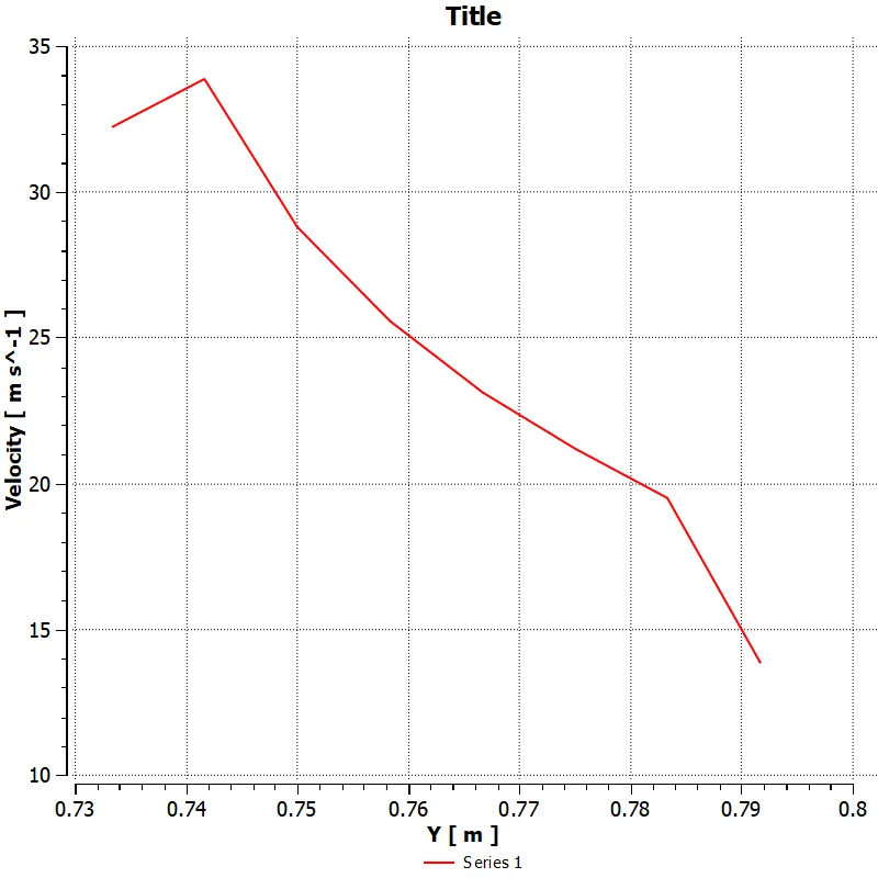
Velocity vs Y(m) :

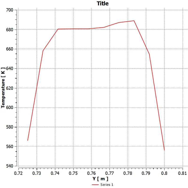
Temperature vs Y(m) :

Velocity contour in Plane 1 :

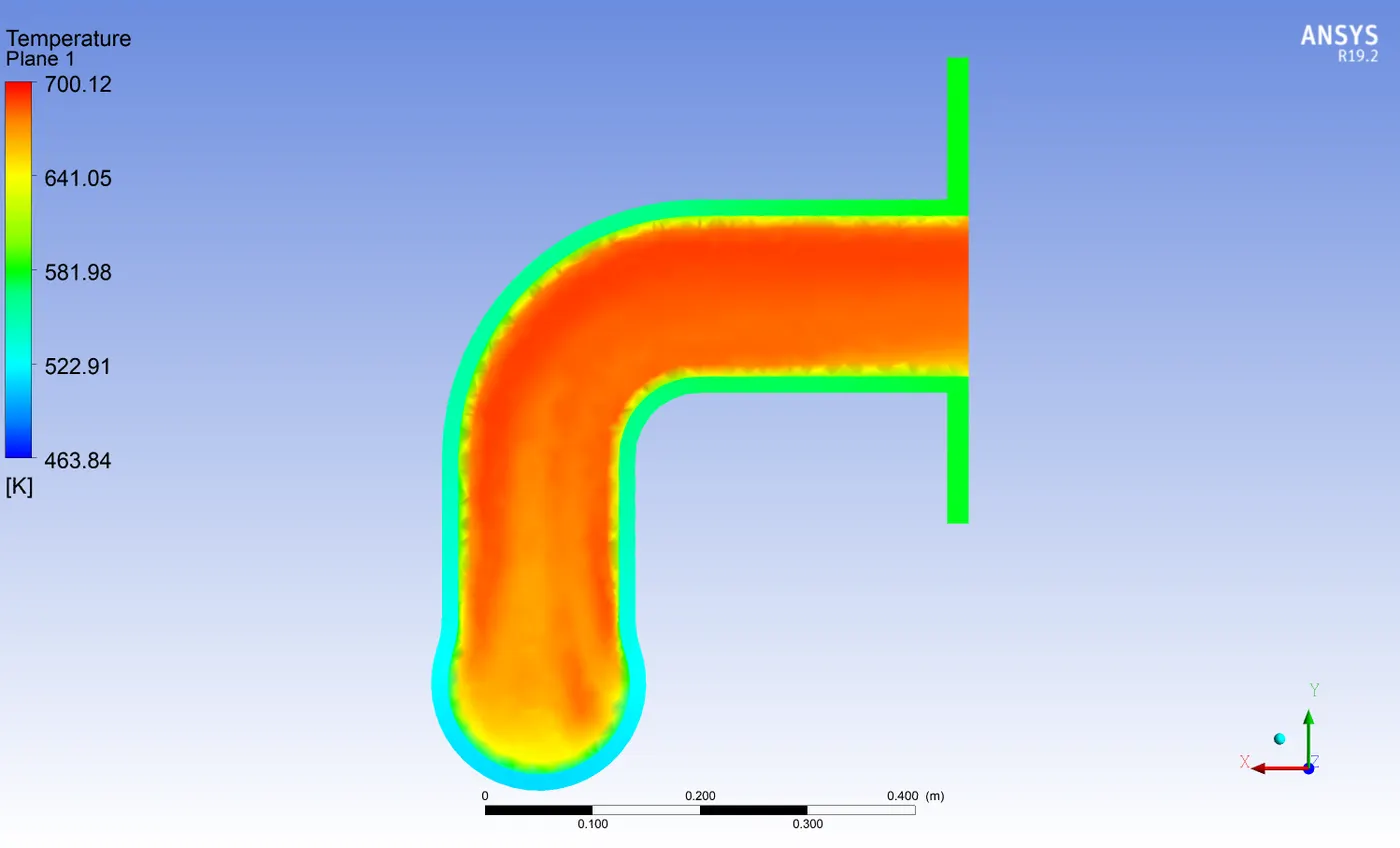
Temperature contour in Plane 1 :

Temperature Contour Animation :

Results:

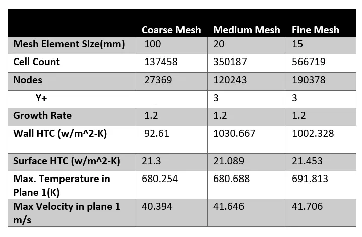
By looking at the results that we have got, we can say that for Base Line Simulation we get diffused results. By refining the mesh, Errors in result got decreased and accuracy was achieved.

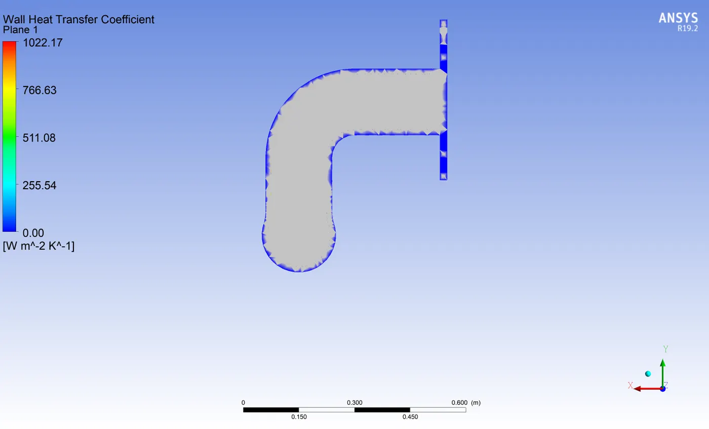
Heat Transfer Coefficient only available on the first cell that is attached to the wall. Since we have added inflation layers in case 2 and 3 we get the smooth looking plot. This smooth looking plot shows a high value of heat transfer coefficient at the first cell location and then that’s where the majority of Heat Transfer is taking place. The reason for adding Inflation Layer is, it creates a Body Fitted Mesh. For our simulation in which flow has strong wall-bounded effects, adding inflation layer is absolutely necessary. We get smooth looking quantity near the wall but for the outer wall lot of Interpolation is going on which leads to the highly irregular looking pattern.

The velocity of the fluid at the region of the lower bend is high, the Higher velocity of fluid will result in higher Reynolds number and high Reynolds number means high Heat transfer from the fluid to solid, this is clearly shown in the contours after simulations are carried out.

Why K-omega turbulence model was chosen:

The k-ε model is more suitable when we are studying free-shear layers and wake region, the standard K-omega model of turbulence is capable of solving turbulence parameters very close to the boundary or wall region. K epsilon is best suited for flow away from the wall, say free surface flow region, whereas the k-omega model is best suited for near the wall-flow region. If we are interested in capturing the phenomenon in-wall region, we have to have very fine meshing near the wall, so the Y+ value is was kept as small as possible. The Y+ value was chosen between 1 and 5.

Verification of the result :

• After successfully carrying out the simulation, The maximum HTC was found out to be 1035 W/m²K and the required heat transfer coefficient was around 970W/m² Since the deviation from the required result is less we can say that the simulation is carried out in a proper way and the result is within an acceptable range.
• By looking at the contours we can say that the velocity is really low in the inlet sections but high in the outlet section, that’s because of mass conservation.

V₁A₁+ V₂A₂+ V₃A₃₊ V₄A₄= V_out A_out

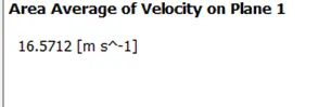
0.81652(5+5+5+5)= V_out

Theoretical V_out=16.3m/s

Simulation output:

• A Nusselt number is a dimensionless number that is used in the study of mass transfer. The Nusselt Number is denoted by the symbol 'Nu'. Since we are going to deal with turbulent flow inside the circular tube, there are two empirical relations on is given by Dittus-Boelter Correlation and another given by Gnielinski Correlation. Dittus-Boelter Correlation is applied when there is a smooth surface and flow is fully developed (Re >10000). Gnielinski Correlation is applied when there is a rough surface and transitional turbulent flow is present.

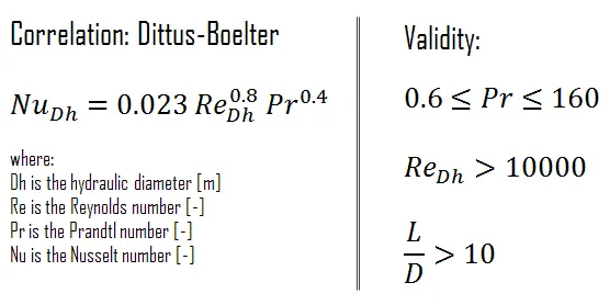
We know,

Nu= hL/K

h can be calculated using the above formula.

From the above equation we can say that when the velocity of fluid increases Reynolds number will increase and since the Nusselt number is directly proportional to the Reynolds number, Nusselt number will increase, increase in Nusselt number means an increase in Heat Transfer. After carrying out the simulation we can observe that at the lower bend of outlet, velocity becomes high and the HTC in that region is also High.

Factor affecting accuracy :

• Y+ : Maintain Y+ between 1-5.
• cell count
• Adding inflation layer around the fluid volume to accurately capture the boundary layer region for wall-bounded turbulent flow.
• Choosing the proper turbulence model.

Conclusion :

Simulations were carried out for 3 different cases and we found out that with refined mesh the results more accurate and efficient. The results obtained were then verified using the Dittus-Boelter equation.