Ahmed Body Challenge
Aim: To simulate the Ahmed body and to calculate the Coefficient of drag and lift.
Introduction :
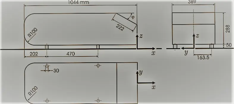
The Ahmed body is a bluff type body that was designed to study the slant angle effect on the cars drag coefficient. It has a simple shape in the entrance region to minimize detachment points in the flow generated by the slant angle. Thus, it is easier to study the wake effect on the drag force. A typical Ahmed body has three different parts. First, the face has rounded corners to adapt the flow in the inlet, so the boundary layer must follow the body shape without flow separations; second, the following part has a rectangular shape to stabilize the flow before the slant angle; and finally, the last part is the slant angle, where the largest separation point is located. In bluff type bodies, the drag force is caused mainly by the pressure field changes. Therefore it is important to relate the drag force to the wake behaviour because it generates the main changes in the pressure field behind the body. It is the benchmark for the aerodynamic simulation tool.
Y plus :

Where y -->Distance from the wall

Is the frictional velocity
The y+ value is a non-dimensional term that can be used to understand how coarse or fine our grid is. This can then be used to determine if wall functions need to be used or not.
The image below shows the boundary layer development
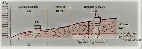
We first start in the laminar region, then transition to the turbulent region. Near the wall, due to the viscous forces, the velocity is dragged to zero and as the boundary layer develops, the velocity will reach free-stream velocity. Turbulent flows have a smaller laminar region near the wall and if we are to resolve the gradients at such a small region, we’d need a very small grid size. This is where the y+ value is helpful. From the image attached above, we need to either be in the viscous sub-layer or the turbulent region. If we were in the viscous sub-layer, that would mean a y+ of less than 10 and if we were in the turbulent region, it would mean a y+ of greater than 30. This is very significant in our making the decision of using or not using a wall function. For a desired y+ value, we can calculate the first cell height. The y+ is not based on the first cell, but the first node. This would be the cell centroid since, for the finite volume method, the cell centre is the node. Using the y+, the way in which velocity is calculated changes. The y+ value gives us an idea of where the first cell centre lies. Using the y+ value, we can understand how exactly we can approach the problem.
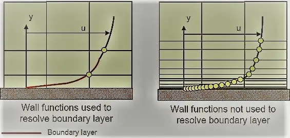
If we refer to the images below, on the left-hand side we observe that the boundary layer profile is modelled with a reduced cell count, which is characteristic of a wall function approach. On the right, the boundary layer profile is resolved all the way to the wall. This will provide a more accurate resolution of the boundary layer. For certain simulations such as flows with strong wall-bounded effects, this resolution is necessary.
Representation of Wall Function approach vs fully resolving the boundary layer
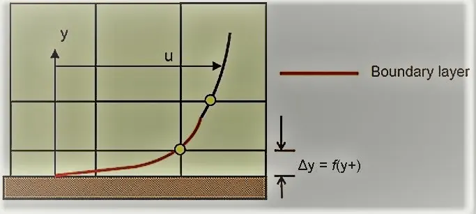
To use a wall function approach for a particular turbulence model with confidence, we need to ensure that our y+ values are within a certain range.
Flow separation :
Flow separation is the detachment of a boundary layer from a surface into a wake. Separation occurs in the flow that is slowing down, with pressure increasing, after passing the thickest part of a streamlined body or passing through a widening passage.
The boundary layer separates when it has travelled far enough in an adverse pressure gradient that the speed of the boundary layer relative to the surface has stopped and reversed direction. The flow becomes detached from the surface and instead takes the forms of eddies and vortices. The fluid exerts constant pressure on the surface once it has separated instead of a continually increasing pressure if still attached. In aerodynamics, flow separation results in reduced lift and increased pressure drag, caused by the pressure differential between the front and rear surfaces of the object.
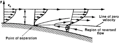
- significance of the point of separation: The point of separation of flow in the car body determines the size of the wake region. If the separation of the flow is occurring early then it would result in large wake region and higher drag force. Increased drag force would affect the fuel efficiency of the vehicle. To achieve a low drag coefficient, optimization in aerodynamic design is done to shift the point of flow separation. In the case of Ahmed body, by adjusting the slant angle we can control the flow separation.
Methodology :
- Creating Geometry :
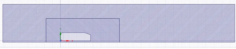
The model is imported to space claim. Initially, a computational fluid domain is created using enclosure option its dimensions are shown below, a second enclosure is created to effectively capture the flow around the Ahmed body. Once both the enclosure is created, it is made sure that there is zero interference so that the generated mesh will be more structured and Share topology is set to share.
Since the Ahmed body which we use is perfectly symmetric, we carryout simulation only on the one half of the body.
2.Meshing :
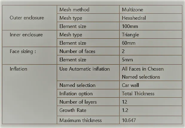
Meshing is the important part to get the accurate results of the experiment. The mesh influences the accuracy, convergence and speed of the simulation. The model is meshed using ANSYS mesher.
Sectional view of the mesh :

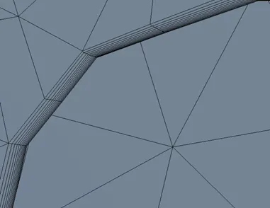
Inflation Layers
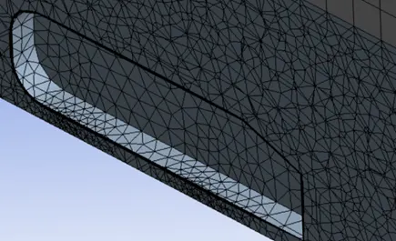
Nodes: 44618
Elements: 117559
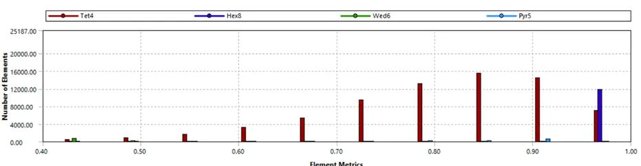
Mesh metrics: Element Quality
The mesh matric that identifies the elements according to their quality was employed, it can be seen that the mesh with low element quality is minimal.
3.Solver Setup :
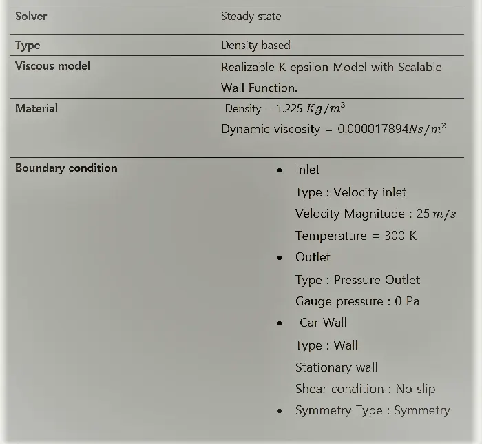
Following are the steps taken for setting up the solving techniques in the solver for 3D, steady-state, incompressible flow using double precision and serial processing technique.
- Import the meshed model created in Workbench and check for the mesh.
- Defining models such as viscous model (Realizable K epsilon Model) is done. A Scalable Wall Function is chosen for near-wall treatment.
Initialize Solution: Solution is initialized from inlet region with set initial values.
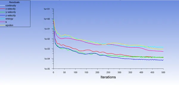
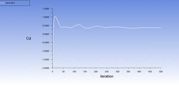
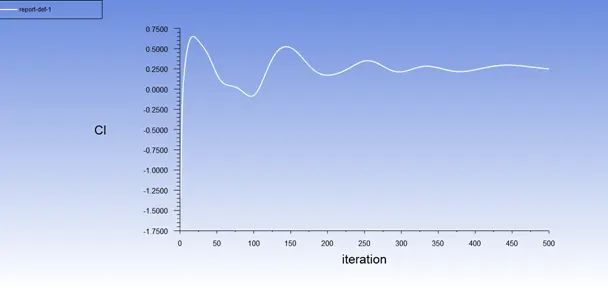
Run calculation: Number of iterations is set to 500 with a reporting interval of 1 (each iteration).
Simulation results:
Residual Plot :
Drag coefficient :
Lift Coefficient:
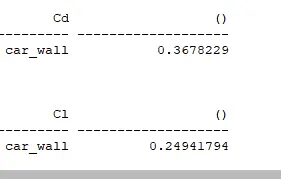
Drag and Lift coefficient values:
Post Processing :
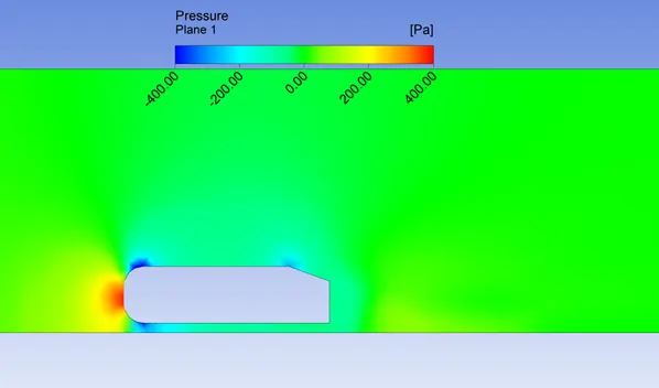
Pressure contour:
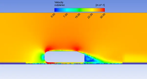
Velocity contour plot:
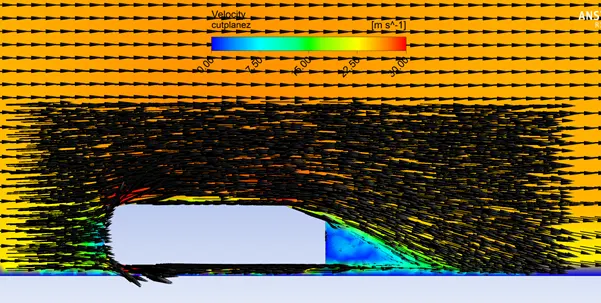
Velocity contour with vectors :
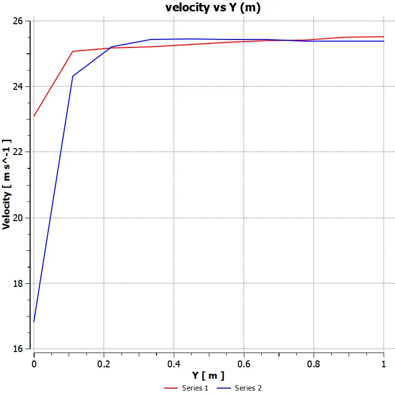
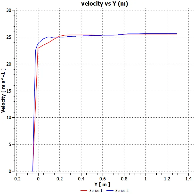
Velocity vs Y chart :
Negative pressure in the wake Region :
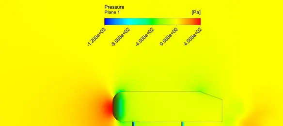
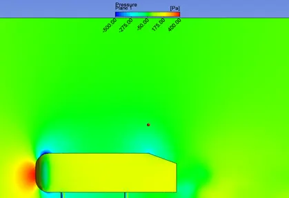
From the Pressure contour plot, it can be observed that there is negative pressure, The sudden change in the boundary of the body leads to the formation of the wake. The flow separation and balancing out of shear stress leads to the negative pressure. As the flow goes towards the rear of the body recirculating zone can be seen. This negative pressure pulls the body and causes an increase in pressure drag.
Grid independency test :
A mesh independence test was undertaken in order to determine the best mesh for the study. It is generally assumed that a higher cell number leads to more accurate results, but a higher cell count in turn leads to longer processing time. Thus, a mesh independence test was undertaken to find a suitable mesh set up which provides acceptable results when simulated by consuming less processing time, K-𝜀 generally considered the fastest of the turbulence models.
Case 1:
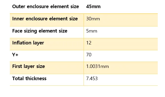
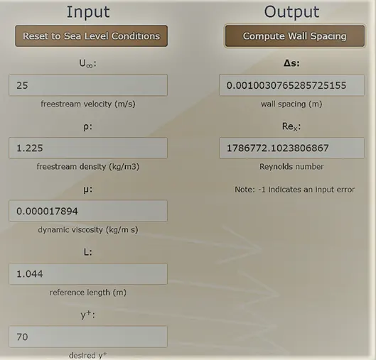
First layer size calculation:
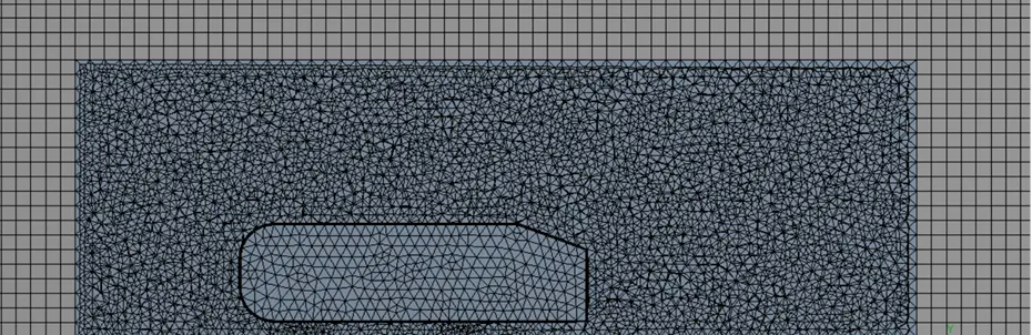
Sectional view of the mesh:
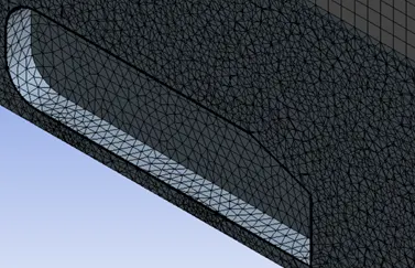
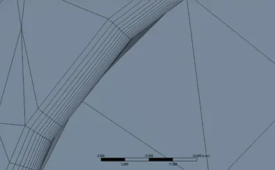
Inflation Layers
Nodes: 245676
Elements:646273
Mesh Metrics: Element quality
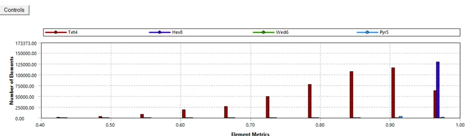
The mesh matric that identifies the elements according to their quality was employed, it can be seen that the mesh with low quality are minimal, most of the elements have very high quality in the range of 0.8-1
No changes are done in the solver setup.
Result plots :
Residual Plot :
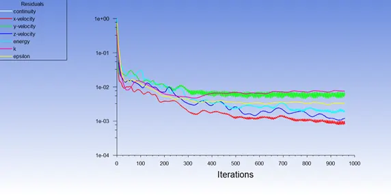
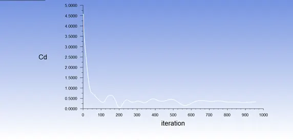
Drag Coefficient plot :
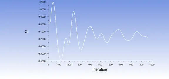
Lift coefficient plot:
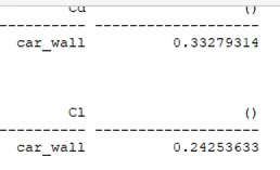
Drag and Lift coefficient value
Pressure Contour plot :
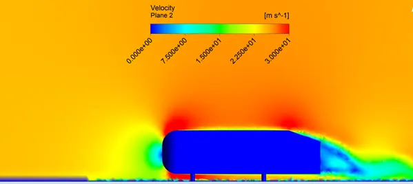
Velocity contour plot :
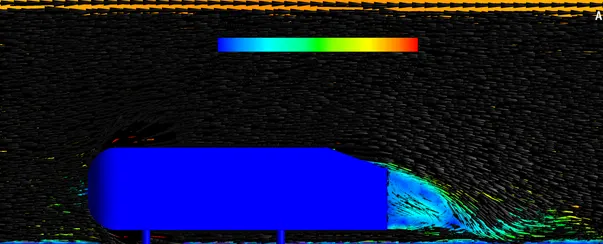
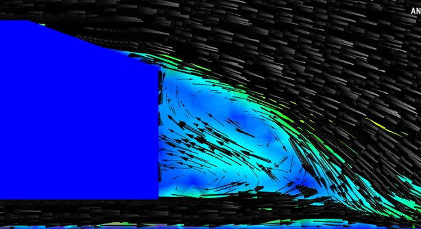
Velocity contour with vectors :
Creating vertical Lines :
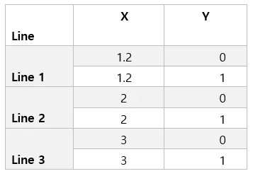
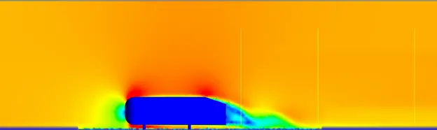
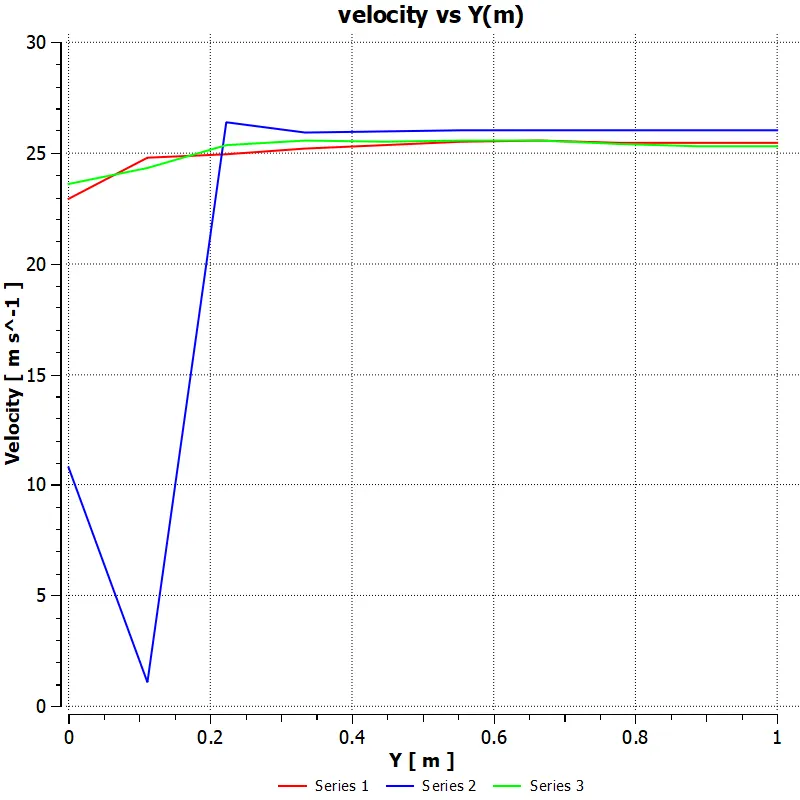
Chart:
Case 2:
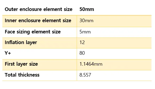
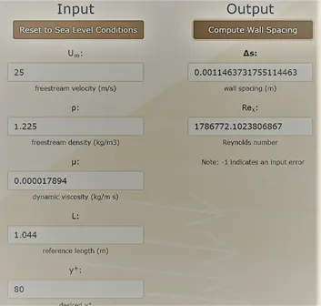
First layer size calculation:
Sectional view of the mesh:
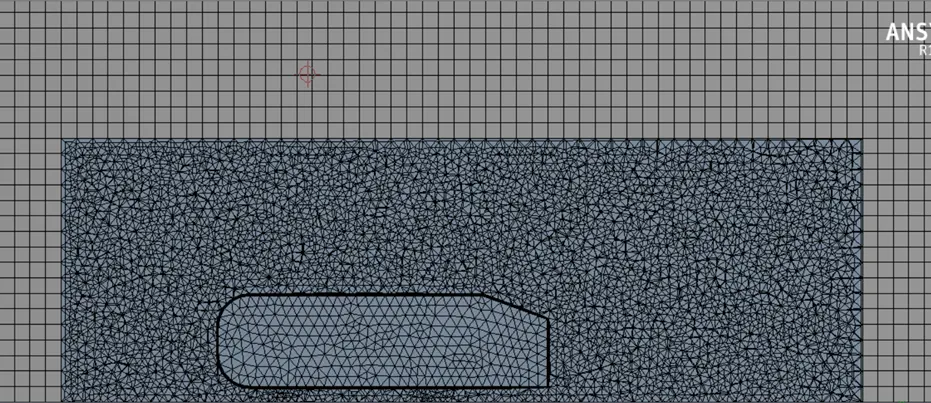
Dimensions of the enclosures remain unchanged.
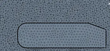
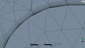
Inflation Layers
Nodes: 213232
Elements:631546
Mesh Metrics: Element quality
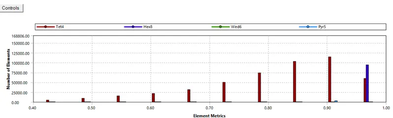
The mesh matric that identifies the elements according to their quality was employed, it can be seen that the mesh with low quality is minimal, most of the elements have very high quality in the range of 0.8-1.
Result plots:
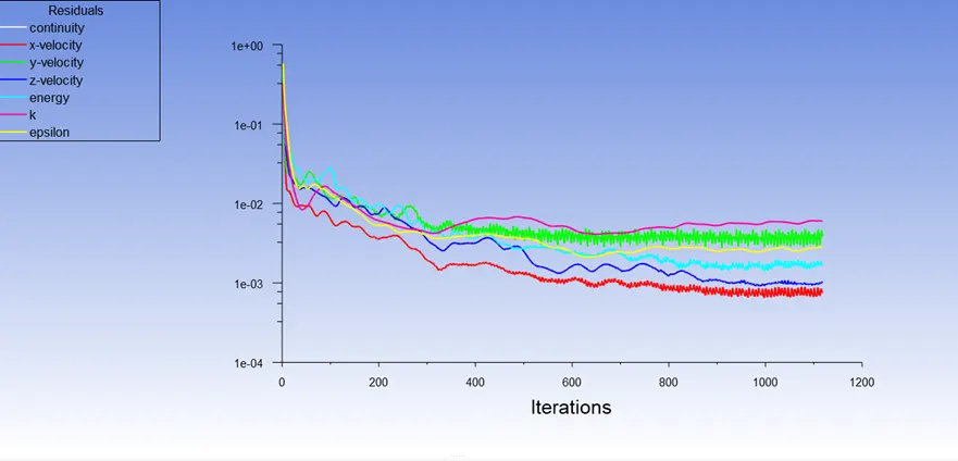
Residual plot:
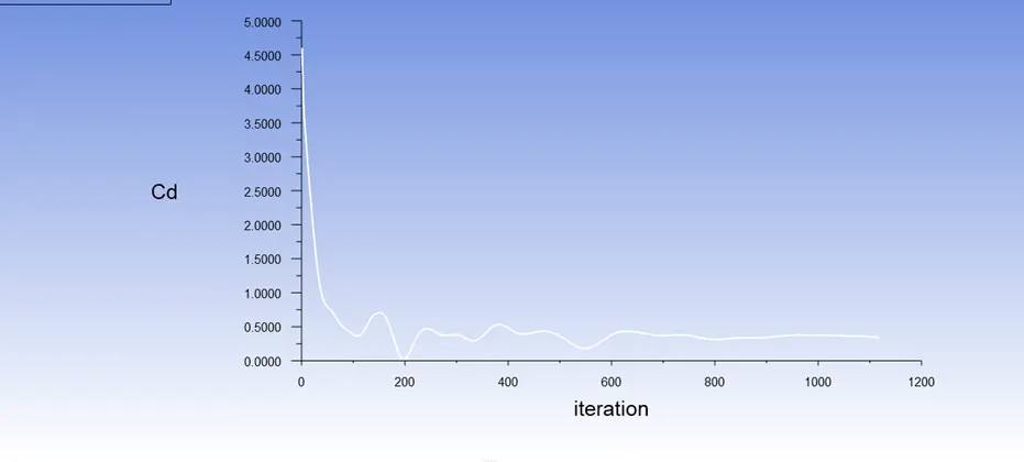
Coefficient of drag plot :
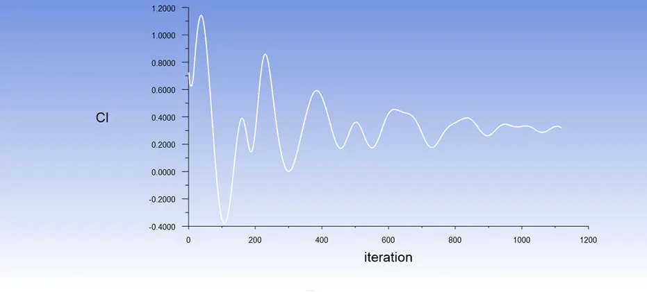
Coefficient of lift plot :
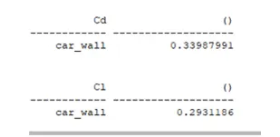
Drag and Lift coefficient values:
Pressure contour plot :
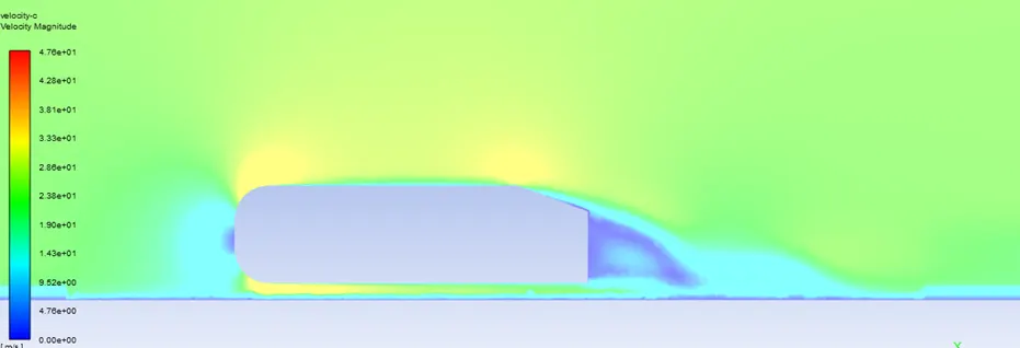
Velocity contour plot :
Velocity contour with vectors :
Car wall variable: Pressure
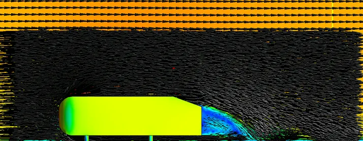
Chart :
Case 3:
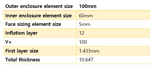
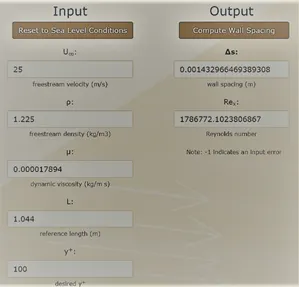
First layer size calculation:
Sectional view of the mesh :
Inflation layers
Nodes: 44618
Elements: 117559
Mesh metrics: Element Quality
The mesh matric that identifies the elements according to their quality was employed, it can be seen that the mesh with low quality are minimal.
Result plots:
Residual plot:
Drag coefficient plot :
Lift coefficient:
Drag and Lift coefficient values:
Pressure contour Plot:
Velocity contour plot :
Velocity contour with vectors :
Chart:
Table:
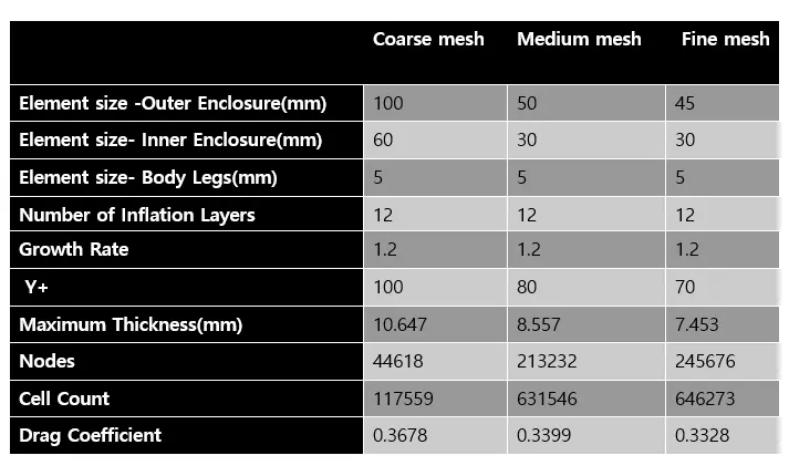
From the results, we could see that the for the Finer mesh drag value is close to the accepted value(0.33), by refining the mesh more appropriate value of drag coefficient can be obtained, as the number of elements increases the accuracy of the result also increases. By looking at the above table we can say that for a Y+ value between 80 and 70 with cell counts between 0.6-0.7 million results obtained will be more accurate.
Conclusion :
Flow Simulation over Ahmed body is successfully carried out and required results are obtained. It is observed that the wake region is formed behind the body which is responsible for the pressure drag, and for better-refined mesh results will be accurate.
---------------------------------------------------------------------------------------------------------------------------------------------------------------------------------------------------------------------------------------------------------------------