Development of a forward energy-based model of a P1 hybrid vehicle

AIM: To develop of a forward energy-based model of a P1 hybrid vehicle by writing MATLAB scripts and modelling in SIMULINK, analysing and generating plots.

OBJECTIVES OF THE PROJECT:
1. To develop a forward energy-based model of a P1 hybrid vehicle which simulates the vehicle on different drive cycles like UDDS, HWFET, FTP, NEDC, etc.
2. A MATLAB script is used to load all the variables required for running the SIMULINK model.
3. The SIMULINK model of the vehicle is modelled using a Driver, Controller and a Powertrain block.
4. The SIMULINK model is executed and data from the model will be loaded in the MATLAB workspace.
5. The MATLAB script used to analyse the SIMULINK model data and to generate the required plots such as,
a. Plotting the time trace for engine, transmission input, transmission output and wheel speeds.
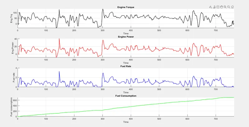
b. Plotting engine torque, engine power, fuel rate and fuel consumption.
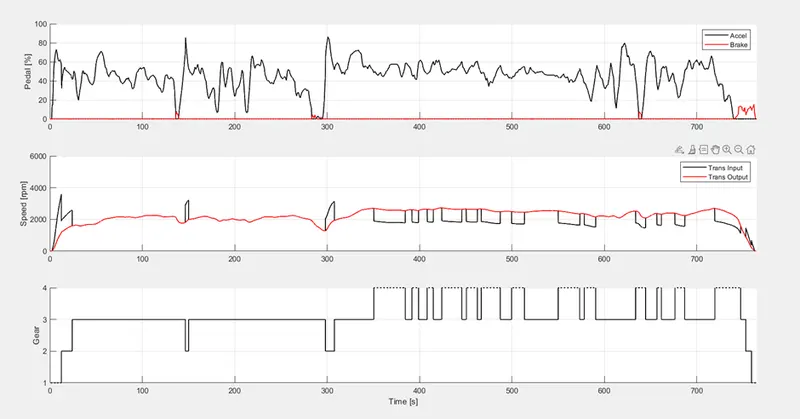
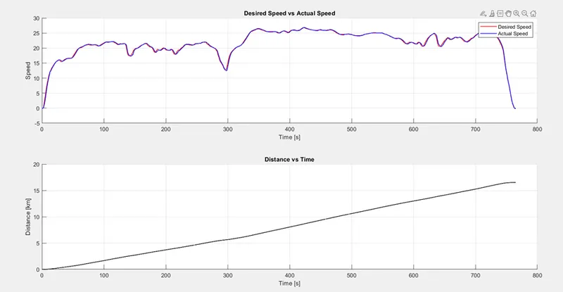
c. Plotting accelerator and brake pedal, gear command, vehicle desired and actual speed, vehicle distance.
d. Plotting the engine operating points on the engine fuel map.
e. Plot motor speed, torque, and motor input power.
f. Plot pack voltage, current and SoC.
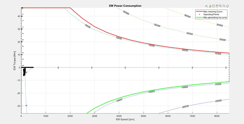
g. Plot the motor operating points on the motor input power map, with the motor max motoring and generating torque curves.

Energy based models

There are two basic types of structure for the energy based models,
i) Forward Model: Dynamic simulation of the system. Simulate from the source to the sink i.e., starts simulation from the input to the engine to the wheels to determine the performance.

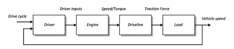
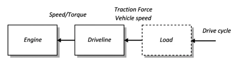
ii) Backward Model: Quasi-Static simulation of the system. Simulate from the sink to the source i.e., input is the vehicle speed and acceleration and the engine input is back calculated.

Hybrid Vehicle: A hybrid vehicle is a vehicle that uses more than one means of energy, basically combining a petrol or diesel engine with an electric motor. Hybridization of vehicles adds functionality such as having a battery charged on the go and the same power can be used to run the accessories as well as boost the performance by providing the initial torque to the transmission. Since the battery gets charged on the go the battery can also power the wheels thereby reducing the load on the engine and the efficiency is boosted. The braking losses that occurred is reduced by the regen braking in the hybrids which adds up the extra range to the vehicle. Hybrid vehicles will generally have two energy sources and converters a bi-directional and a unidirectional. The bi-directionality of one powertrain gives multiple energy flow paths thereby increasing flexibility. Based on the design and flexibility of the hybrid powertrain there are structurally different types of hybrid vehicles. In Mild hybrid vehicles (MHEV) (such as Honda insight in our project) The electric motor can be positioned, relative to the other powertrain components, in five major points:

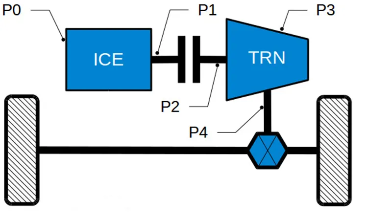
A brief description of the electric motor connection points is shown below.

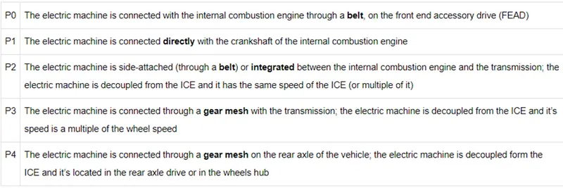
The P1 architecture, with the electric machine connected directly to the crankshaft, is the solution adopted by Honda on their first-generation Integrated Motor Assist (IMA) technology. The electric motor functions as a generator, during vehicle deceleration, as an engine starter, and as a motor (to assist the engine) during vehicle accelerations.

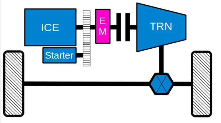
One of the biggest advantages of this solution is that the electric motor can provide higher torque. However, since there is no speed/torque ratio between the electric machine and the crankshaft, the torque requirements on the electric motor can be quite demanding.

One of the example for P1 MHEV architecture is:

Honda Insight Hybrid 2009 (with Integrated Motor Assist technology)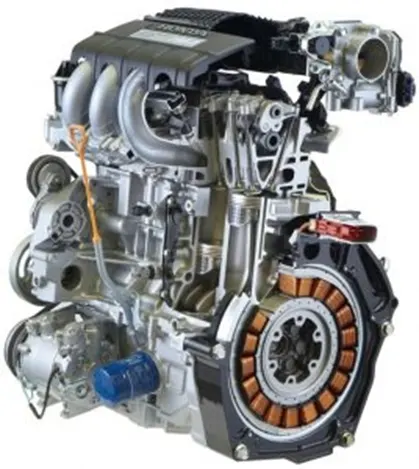

P1 HYBRID VEHICLE FORWARD MODEL

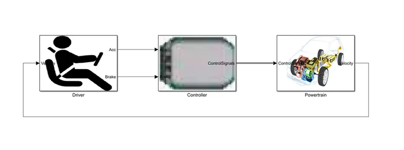
The model consists of 3 main blocks such as Driver, Controller and Powertrain as shown in above figure. The Driver block is a basic PI controller which generates the accelerator and brake pedal outputs required to match the desired and actual vehicle speed.

DRIVER MODEL

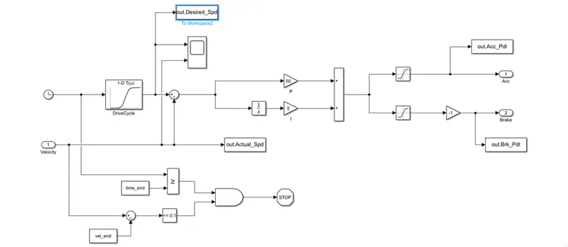
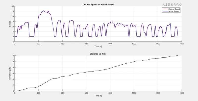
The drive cycle data is fed as input in the driver block and the feedback velocity is given from the powertrain block. The lookup table consists of the drive cycle data, desired speed as a function of time. The positive speed values are given out as acceleration output and the negative speed values are given as brake outputs. The scope block in this subsystem is to check the desired speed and the actual speed. The output of the scope block is shown below. The vehicle velocity traces the drive cycle speed with minimum overshoot and upper shoot. (For UDDS cycle)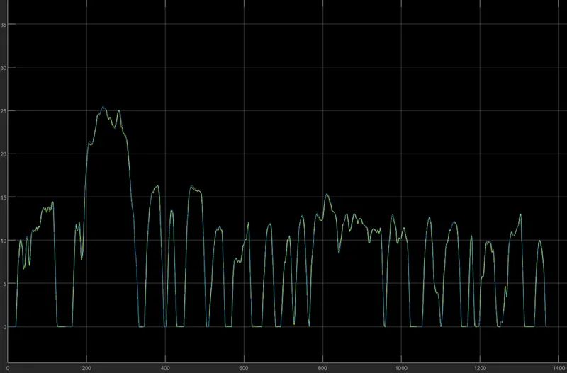

Controller

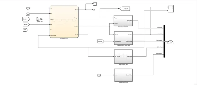
The Controller block represents the electronic control unit of the vehicle. It works based on the driver inputs, it generates desired engine torque, desired transmission gear, desired brake torque, application of the E motor and locking up the clutch. The outputs from the driver block which are the acceleration and brake pedal signals are passed on to the Controller block. The block contains subsystems namely, the Engine control unit, the Transmission control unit, the E motor control unit and the brake control unit along with the state chart for mode selection whose outputs are fed to the powertrain block.

Mode selection block shown below is a state chart which takes the inputs such as accelerator and brake pedal, engine speed, velocity, SOC and clutch lock up. The outputs from this chart are mode, engine on or off, amount of engine throttle and amount of E motor throttle. The mode selection consists of various states inside it which is shown below.

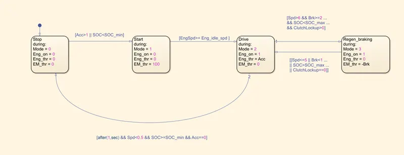
The mode selection consists of 4 modes stop, start, drive and regen braking. The transition from the states takes place if the conditions mentioned along the transition line are met.

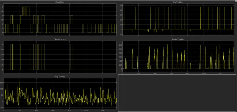
The figure below shows the output of scope block in the controller which shows the time traces of engine torque required which is output of engine control unit, gear command the output of transmission control unit and the E motor torque required the output of E motor control unit along with the clutch lock up.

Engine Control
The engine control unit takes the input throttle and Engine on (which will be 0 or 1) which is the accelerator output from the driver block. The throttle is added with the output of the idle speed controller block which basically maintains the engine speed not to drop below the engine idle speed.

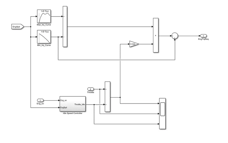
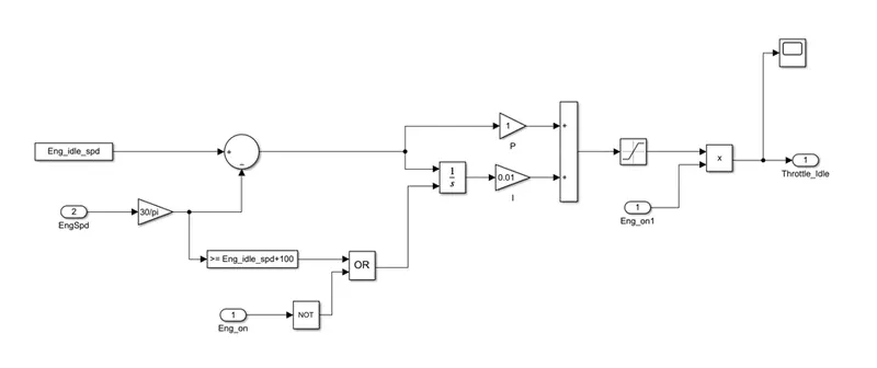
Idle speed controller also has a PI controller to maintain the engine speed. Also it makes the engine speed 0 when the input from the engine on port is 0. There by switching off the engine instead of running in idle speed. The engine control unit takes the feedback of engine speed and then generates the torque required as output.

Idle Engine Speed controller

Transmission Control

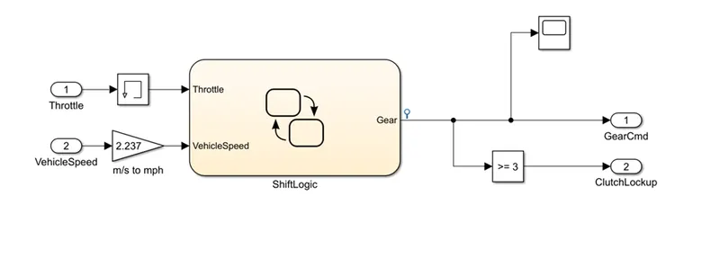
The transmission control unit takes the inputs such as throttle and vehicle speed and provides the output as gear command which indicates the gear at which the vehicle is operating. Also when the vehicle is at 3^rd gear the clutch is locked up there by giving us the output in form of 0 or 1. This subsystem uses a Stateflow which is shown as a shiftlogic in the above figure.

Shift logic

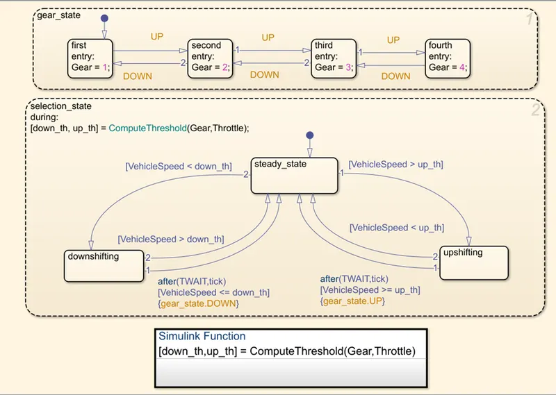
Stateflow is a graphical environment for decision logic modelling, the gear state is a super state and the selection state is the substate. The gear state has four states representing the four gears of the vehicle. The substate selection state is entered and based on the logic whether the vehicle speed is greater or lesser the transition occurs. If the vehicle speed is greater than the up threshold then the transition (UP) occurs and the gear shifts to the next state (i.e., from gear1 to gear2). Similarly, the transition (DOWN) occurs if the vehicle speed is less than the down threshold. These thresholds are specified as s SIMULINK function.

EM(Electric Motor) Control unit

Since there is a E motor running with the engine a control unit is required to control the operation of the motor the motor runs at the same speed of the engine.

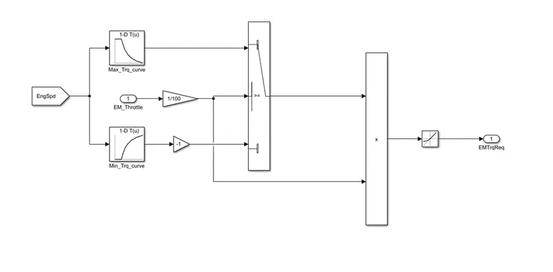
The E motor speed goes through the 1 d look up table and gives the torque required, the negative speed is when the regenerative braking is happening.

Brake Control

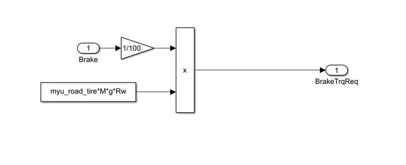
The Brake pedal signal from the driver block is multiplied by the maximum friction, which gives the maximum braking torque. The required break torque is calculated as output.

Power Train

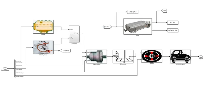
The Powertrain block consists of subsystems like Engine, Electric motor, crack hub, Energy storage system, Transmission, Differential, Wheels and Vehicle Dynamics. The inputs to the powertrain is given by the outputs from the controller block such as the engine torque and E motor torque required is fed to the engine block and Electric motor block respectively and the gear command along with clutch lockup is fed to the transmission block and the brake torque required is fed to the wheels. The output from the powertrain block is the velocity which is fed back to driver block as a feedback.

Engine

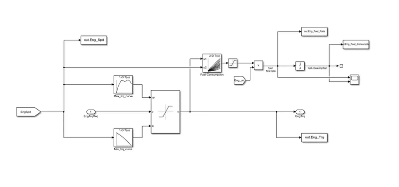
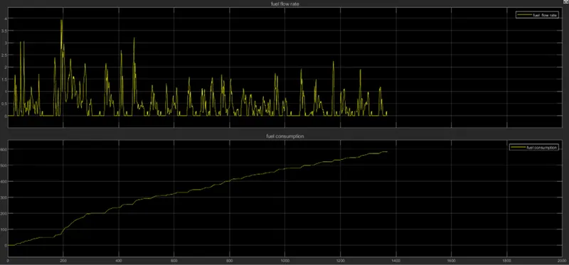
The engine block takes the input as engine torque required from the engine control unit and it is compared with the maximum and minimum torque and maintained between the required range using the dynamic saturation block. Further, with both the engine torque and the engine speed the fuel consumption rate is found through a 2-D lookup table. The saturation block is implemented to take only the positive values. Further, the value is multiplied with the Engine on parameter which will be 1 for engine on and 0 for engine off. On integrating the engine fuel consumption is determined which is sent to the MATLAB workspace for plotting purposes. The scope block shows the time trace of the fuel flow rate and engine fuel consumption which is shown below.

Electric Motor

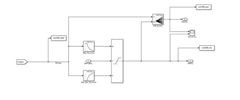
The Electric motor takes the input of electric motor torque request from the electric motor control unit and based on the look up tables gives out the output of electric power and torque required. The content inside the Electric motor is shown below.

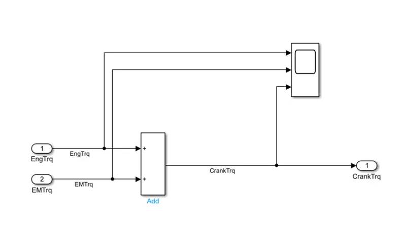
Further, both the torques the engine torque and the E motor torque are added in the crank hub block which is shown below.

Transmission

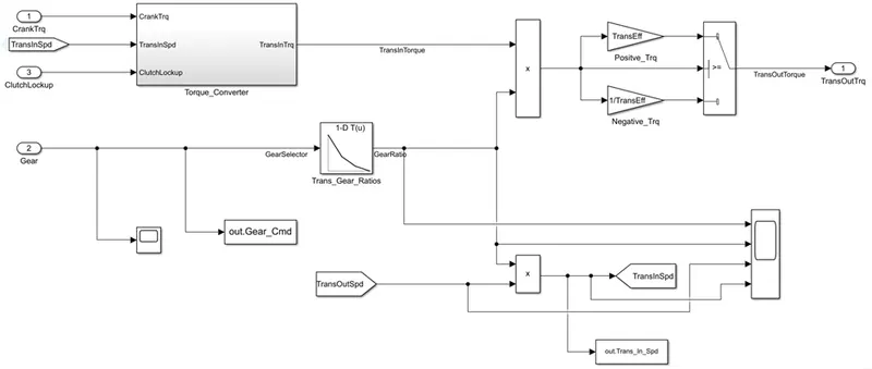
The transmission block takes the input as crank torque from the output of the crank hub block and the gear and clutch lock up as input from the transmission control unit. Further, the signal is passed to the torque converter block which gives out transmission in torque for the selected gear the gear ratio is multiplied to the output from torque converter.

Torque converter

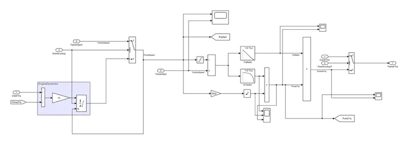
It takes the inputs as crank torque, transmission in speed and clutch lock up. When the clutch is locked up the pump speed is the engine speed and when the clutch is not locked the turbine speed is divided by the pump speed on further calculations the turbine torque is determined which is given out as transmission in torque.

ESS (Battery)

As the fuel is supplied to the engine from the fuel tank similarly the electric power is supplied to the motor from the batter system. This system is known as Energy Storage System as the name says it stores the energy in the from of electric power. The block takes the input as electric power from the E motor block. The content of the block is shown below.

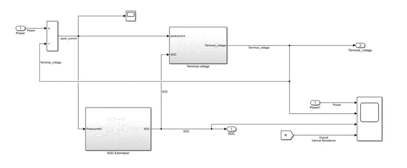
The electric power fed as input is used to calculate the pack current further this pack current is fed to SOC block to determine the state of charge.

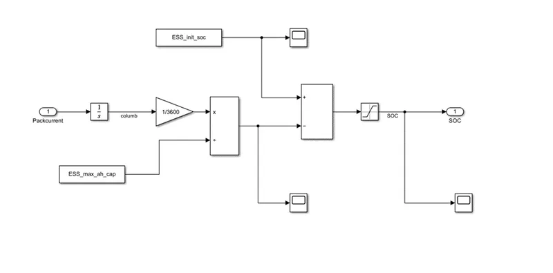
The pack current which is fed in is converted in form of amp-hr and then divided by the max current capacity which gives the used SOC. By subtracting the initial SOC by used SOC the remaining SOC at that time interval is determined. The saturation block saturated the SOC between 0 and 1

The soc and the pack current are fed as inputs to terminal voltage block to determine the terminal voltage.

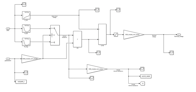
This block takes pack current and SOC as inputs. The internal resistances while charge and discharge conditions (based on positive and negative pack current) are determined using a 1-D lookup table and switch block. The current is divided by the number of modules in parallel and further is multiplied by internal resistance (I*R). Using another 1-D lookup table the open circuit voltage is determined. Further for terminal voltage,

Terminal voltage = open circuit voltage – (pack current*internal resistance)

Differential

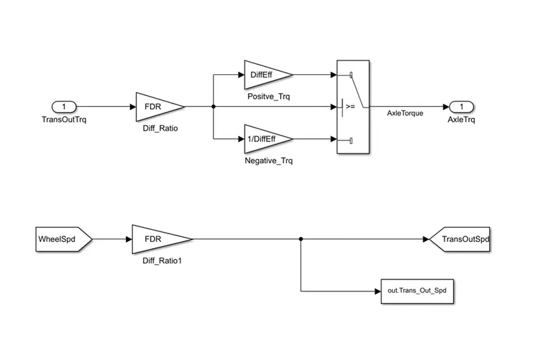
The Differential block takes the input as transmission out torque and computes it by multiplying with differential ratios and the output is given as axle torque. In the same block the transmission out speed is calculated by multiplying the wheel speed with the differential ratio.

Wheels

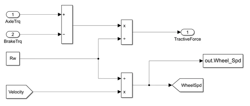
The wheels take the inputs as axle torque and brake torque, where the brake torque is subtracted from the axle torque and divided the rolling friction constant to get Tractive force as output. Similarly on dividing the velocity by the rolling friction constant gives the wheel speed.

Vehicle Dynamics

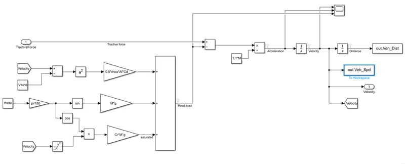
The output from the wheels block which is the tractive force is subtracted by the road load, further on dividing by mass the acceleration is obtained. On integrating the acceleration the velocity is obtained and further integrating it will provide the distance travelled.

The equation for modelling the vehicle dynamic block is shown below,

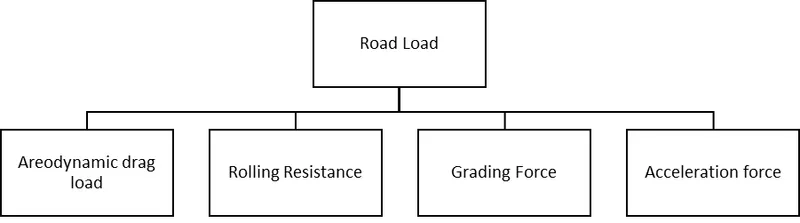
The input variables and system parameters that would be required to calculate the power requirement and energy consumption of the system.
The aerodynamic force is given by,

F_ad = Aerodynamic drag force
ρ = Density of air
A_f = Frontal area
C_d = Drag coefficient
V_vh = Vehicle velocity
V_w = Wind velocity

The Rolling resistance is given by,

F_rr = Rolling force
M = Mass of the vehicle
g = acceleration due to gravity
C_r = rolling coefficient
ϴ = angle of inclination

The grade force is given by,

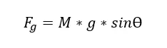
F_g = Grading force
M = Mass of the vehicle
g = acceleration due to gravity
ϴ = angle of inclination

Acceleration force is given by,

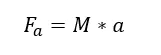
F_a = Acceleration force
M = Mass of the vehicle
a = acceleration

MATLAB INITILIZATION CODE:

In this project, a typical midsize car with a 1.9L engine and a 4-speed automatic transmission with a Permanent Magnet Synchronous Motor of 10kW and 6Ah 154V NiMH battery pack is considered. Data is taken from ADVISOR data base developed by NREL, USA. Transmission shift map and controller is taken from MATLAB/SIMULINK example database. The model developed has the capability to simulate the vehicle on different drive cycles like UDDS, HWFET, FTP, NEDC, etc. The file “Project2_InitFile.m” is a MATLAB script used to load the variables to run the SIMULINK model. Also, the code prompts the user to select the required drive cycle for simulation.

%%%%%%%%%%%%%%%%%%%%%%%%%%%%%%%%%%%%%%%%%%%%%%%%%%%%%%%%%%%%%%%%%%%%%
%% Skill-Lync -> Hybrid Drives Development
% Project 2 - P1 hybrid Vehicle Model


% Description:

%% Initialization File
% Initialization file for loading the variables for the P1 hybrid Vehicle Model Simulation

clear all
close all 
clc
%% Vehicle Parameters
M = 1500;       % Vehicle weight [kg]
Cr = 0.015;     % Rolling resistance coefficient
Rw = 0.35;      % Rolling radius [m]
Cd = 0.33;      % Drag coefficient
Af = 2;         % Frontal area [m2]
rhoa = 1.225;   % Air density [kg/m3]
Vwind = 0;      % Wind velocity [kmph]
g = 9.81;       % Gravitational acceleration [m/s2]
theta = 0;      % Slope [deg]
myu_road_tire = 1; % Coefficient of friction between tire - road interface

%% Powertrain Parameters 
FDR = 3.73;                         % Final Drive Ratio / Diff Ratio
DiffEff = 0.99;                     % Differential efficiency (assumed independent of operating conditions)

NumGear = 4;                        % Number of gears in transmission
TransGear = [1:NumGear];            % Transmission Gears
TransRatio = [3.06, 1.62, 1, 0.7];  % Corresponding Transmission ratios
TransEff = 0.90;                    % Transmission efficiency (assumed independent of operating conditions)

TC_SR = [0, .5, .6, .7, .8, .87, .92, .94, .96, .97, 1];   % Torque Converter Speed Ratio (Matlab default) -> TurbSpd/PumpSpd  
TC_TR = [2.232, 1.5462, 1.4058, 1.2746, 1.1528, 1.0732, 1.0192, 1, 1, 1, 1];   % Torque Converter Torque Ratio (Matlab default) -> TurbTrq/PumpTrq
TC_Cf = 1e-4 * [.72558, .66322, .63463, .59042, .51331, .4144, .29287, .22444, .12186, .04386, 0]; % Torque Converter Capacity Factor (Matlab default) -> PumpTrq/PumpSpd^2 [Nm/rpm^2]

load Vehicle_Data/Engine_data_1_9L_Saturn_95kW
load Vehicle_Data/Trans_Shift_map
load Vehicle_Data/EM_Honda_Insight_10kW
load Vehicle_Data/ESS_NiMH6


ESS_init_soc = 0.8;         % Initial state of charge
ESS_soc_max = 0.9;          % Maximum state of charge
ESS_soc_min = 0.6;          % Minimum state of charge


%% Driver Parameters
Kp = 10;                    % P gain for driver PI model
Ki = 1;                     % I gain for driver PI model
Drive_Cycle_Select = input(sprintf('Drive cycle for Simulation: n1. UDDS n2. HWFET n3. FTP n4. US06 n5. NEDC n6. WLTP nYour selection:'));     % Drive cycle selection

% Drive cycle values in m/s

if Drive_Cycle_Select == 1
    load DriveCycles/UDDS;
    
elseif Drive_Cycle_Select == 2
    load DriveCycles/HWFET;
    
elseif Drive_Cycle_Select == 3
    load DriveCycles/FTP;
    
elseif Drive_Cycle_Select == 4
    load DriveCycles/US06;
    
elseif Drive_Cycle_Select == 5
    load DriveCycles/NEDC;
    
elseif Drive_Cycle_Select == 6
    load DriveCycles/WLTP;
 
end

time_end = cyc_time(end);
vel_end = cyc_vel(end);

MATLAB Post processing code

The SIMULINK model is executed and in order to analyse and plot the required plots the MATLAB script shown below is executed. The outputs from the SIMULINK model are stored in variables in MATLAB and the same are used for plotting.

%%%%%%%%%%%%%%%%%%%%%%%%%%%%%%%%%%%%%%%%%%%%%%%%%%%%%%%%%%%%%%%%%%%%%
%% Skill-Lync -> Hybrid Drives Development
% Project 2 - P1 hybrid Vehicle Model


% Description:
% The following file is to used with the Initialization file and Simulink
% results for post-processing of the data.


%% Post-Processing File
%  File for post-processing the P1 hybrid vehicle simulation model data
close all
clc
%% Renaming variables
Time = out.out_time;
Acc_Pdl = out.Acc_Pdl;          % Accelerator pedal [%]
Brk_Pdl = out.Brk_Pdl;          % Brake pedal [%]
Gear_Cmd = out.Gear_Cmd;        % Transmission gear
Trans_In_Spd = out.Trans_In_Spd*30/pi;  % Transmission input speed [rpm]
Trans_Out_Spd = out.Trans_Out_Spd*30/pi;% Transmission output speed [rpm]
Eng_Trq = out.Eng_Trq;          % Engine brake torque [Nm]
Eng_Spd = out.Eng_Spd*30/pi;    % Engine speed [rpm]
Eng_Fuel_Consump = out.Eng_Fuel_Consumption;    % Engine fuel consumption [g]
Veh_Dist = out.Veh_Dist/1000;   % Distance traveled by vehicle [km]
Veh_Spd = out.Veh_Spd*18/5;     % Vehicle speed [kmph]
Wheel_Spd = out.Wheel_Spd*18/5; % Wheel speed [kmph]
Fuel_rate = out.Eng_Fuel_Rate;  % Fuel flow rate
Fuel_consumption = out.Eng_Fuel_Consumption; % Fuel consumption
Desired_Spd = out.Desired_Spd;  % Desired Speed
Actual_Spd = out.Actual_Spd;    % Actual Speed

% EM Data
EM_Pwr = out.EM_pwr;            % Electric motor Power
EM_Spd = out.EM_Spd;            % Electric motor Speed
EM_Trq = out.EM_trq;            % Electric motor Torque
Elec_pwr = out.ElecPwr;
pack_i = out.pack_i;            % Pack current in Amps
term_volt = out.term_volt;      % Treminal voltage
soc = out.soc;                  % State of Charge


%% Data Analysis
Eng_Pwr = Eng_Spd*pi/30.*Eng_Trq/1000;      % Engine brake power [kW] % Element wise operator added
rho_petrol = 0.7197;                        % Density of petrol [kg/L]
kmpl = Veh_Dist(end)/(Eng_Fuel_Consump(end)/1000/rho_petrol);    % Fuel economy [kmpl] 


%% Plotting vehicle characteristics time trace
figure('name',"Time Traces")
hold on
grid on
plot(Time,Eng_Spd,'LineWidth',1,'color','b')
plot(Time,Trans_In_Spd,'LineWidth',1,'color','r')
plot(Time,Trans_Out_Spd,'LineWidth',1,'color','g')
plot(Time,Wheel_Spd,'LineWidth',1,'color','m')
xlabel('Time')
legend('Engine Speed','Trans In Speed','Trans Out Speed','Wheel Speed')

figure('name',"Engine torque, power, fuel rate & fuel consumption")
subplot(4,1,1)
hold on
grid on
plot(Time,Eng_Trq,'LineWidth',1,'color','k')
xlabel('Time')
ylabel('Eng Trq')
xlim([0, Time(end)]);
title('Engine Torque')

subplot(4,1,2)
hold on
grid on
plot(Time,Eng_Pwr,'LineWidth',1,'color','r')
xlabel('Time')
ylabel('Eng Power')
xlim([0, Time(end)]);
title('Engine Power')

subplot(4,1,3)
hold on
grid on
plot(Time,Fuel_rate,'LineWidth',1,'color','b')
xlabel('Time')
ylabel('Fuel rate')
xlim([0, Time(end)]);
title('Fuel Rate')

subplot(4,1,4)
hold on
grid on
plot(Time,Fuel_consumption,'LineWidth',1,'color','g')
xlabel('Time')
ylabel('Fuel consumption')
xlim([0, Time(end)]);
title('Fuel Consumption')

% Plot of accleerator brake pedal, gear command and transmission speeds
figure('name',"Accelerator brake pedal, gear command & transmission speeds")
subplot(3,1,1)
hold on
grid on
plot(Time, Acc_Pdl, 'linewidth', 1, 'Color', 'black');
plot(Time, Brk_Pdl, 'linewidth', 1, 'Color', 'red');
ylabel('Pedal [%]')
xlim([0, Time(end)]);
legend('Accel','Brake');
subplot(3,1,2)
hold on
grid on
plot(Time, Trans_In_Spd, 'linewidth', 1, 'Color', 'black');
plot(Time, Trans_Out_Spd, 'linewidth', 1, 'Color', 'red');
ylabel('Speed [rpm]')
xlim([0, Time(end)]);
ylim([0, 6000]);
legend('Trans Input','Trans Output');
subplot(3,1,3)
hold on
grid on
plot(Gear_Cmd, 'linewidth', 1, 'Color', 'black');
xlim([0, Time(end)]);
xlabel('Time [s]');
ylabel('Gear');

% Plot of Actual speed and Desired speed
figure('name',"Actual speed, Desired speed & Distance")
subplot(2,1,1)
hold on
grid on
plot(Time, Desired_Spd, 'linewidth', 1, 'Color', 'r');
plot(Time, Actual_Spd, 'linewidth', 1, 'Color', 'b');
xlabel('Time [s]');
ylabel('Speed');
legend('Desired Speed','Actual Speed')
title('Desired Speed vs Actual Speed')

subplot(2,1,2)
hold on
grid on
plot(Time, Veh_Dist, 'linewidth', 1, 'Color', 'black');
xlabel('Time [s]');
ylabel('Distance [km]');
title('Distance vs Time')


%% Plotting engine operating points on engine fuel map
figure('Name','Engine Operating Points');
hold on
grid on
title('Engine Operating Points','fontsize',12);
p1=plot(Eng_map_spd*30/pi,Eng_max_trq,'linewidth',2,'color','r');
p2=line([Eng_map_spd(end)*30/pi Eng_map_spd(end)*30/pi],[0 Eng_max_trq(end)]);
set(p2,'linewidth',1,'linestyle','--','color','k');
p3=line([Eng_map_spd(1)*30/pi Eng_map_spd(1)*30/pi],[0 Eng_max_trq(1)]);
set(p3,'linewidth',1,'linestyle','--','color','k');
[c,h] = contour(Eng_map_spd'*30/pi,Eng_map_trq,Eng_fuel_map');
clabel(c,h);
xlabel('Engine Speed [rpm]');
ylabel('Engine Torque [Nm]');
title('Engine Fuel Consumption Map [g/s]');
p4 = plot(Eng_Spd,Eng_Trq,'.','MarkerSize',0.1,'color','k');
legend([p1 p4],{'Max Curve','Operating Points'});
axis([Eng_map_spd(1)*30/pi Eng_map_spd(end)*30/pi 0 Eng_map_trq(end)]);

%% Electric Motor plots
figure('name',"EM Speed, torque, power")
subplot(3,1,1)
hold on
grid on
plot(Time,EM_Spd,'LineWidth',1,'color','k')
xlabel('Time')
ylabel('Speed')
xlim([0, Time(end)]);
title('EM Speed')

subplot(3,1,2)
hold on
grid on
plot(Time,EM_Trq,'LineWidth',1,'color','r')
xlabel('Time')
ylabel('Troque')
xlim([0, Time(end)]);
title('EM Torque')

subplot(3,1,3)
hold on
grid on
plot(Time,EM_Pwr,'LineWidth',1,'color','b')
xlabel('Time')
ylabel('Power')
xlim([0, Time(end)]);
title('EM Power')

% Plot of current voltage and SOC
figure('name',"Time trace of current, voltage & SOC")

subplot(3,1,1)
plot(Time,pack_i,'linewidth',1,'color','b')
xlabel('Time')
ylabel('Pack Current')
title('Time vs Current')
hold on
grid on

subplot(3,1,2)
plot(Time,term_volt,'linewidth',1,'color','r')
xlabel('Time')
ylabel('Voltage')
title('Time vs Voltage')
hold on
grid on

subplot(3,1,3)
plot(Time,soc,'linewidth',1,'color','g')
xlabel('Time')
ylabel('SOC')
xlim([0, Time(end)]);
ylim([min(soc), max(soc)]);
title('Time vs SOC')
hold on
grid on

%% Plotting Electric Motor operating points
figure('Name','EM Operating Points');
hold on
grid on
title('EM Operating Points','fontsize',12);
p1=plot(EM_map_spd*30/pi,EM_max_trq,'linewidth',2,'color','r');
p5=plot(EM_map_spd*30/pi,EM_max_gen_trq,'linewidth',2,'color','g');
p2=line([EM_map_spd(end)*30/pi EM_map_spd(end)*30/pi],[EM_max_gen_trq(end) EM_max_trq(end)]);
set(p2,'linewidth',1,'linestyle','--','color','k');
p3=line([EM_map_spd(1)*30/pi EM_map_spd(1)*30/pi],[EM_max_gen_trq(1) EM_max_trq(1)]);
set(p3,'linewidth',1,'linestyle','--','color','k');
[c,h] = contour(EM_map_spd'*30/pi,EM_map_trq,EM_inpwr_map');
clabel(c,h);
xlabel('EM Speed [rpm]');
ylabel('EM Torque [Nm]');
title('EM Power Consumption');
p4 = plot(EM_Spd,EM_Trq,'*','MarkerSize',2.5,'color','k');
legend([p1 p4 p5],{'Max motoring Curve','Operating Points','Max generating trq curve'});
axis([EM_map_spd(1)*30/pi EM_map_spd(end)*30/pi EM_map_trq(1) EM_map_trq(end)]);

fprintf('Fuel economy for the selected cycle is: %f kmpl',kmpl)

On executing the above script for UDDS drive cycle

a. Time trace for engine, transmission input, transmission output and wheel speeds.

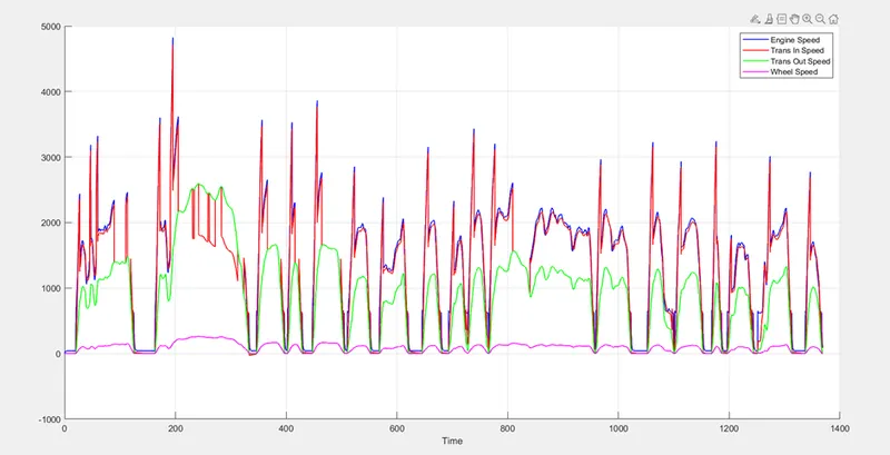
From the above figure we can see the loss occured while the engine speed is transmitted to wheels.

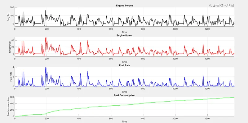
b. Plotting engine torque, engine power, fuel rate and fuel consumption.

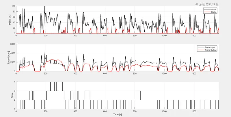
c. Plotting accelerator and brake pedal, gear command, vehicle desired and actual speed, vehicle distance.

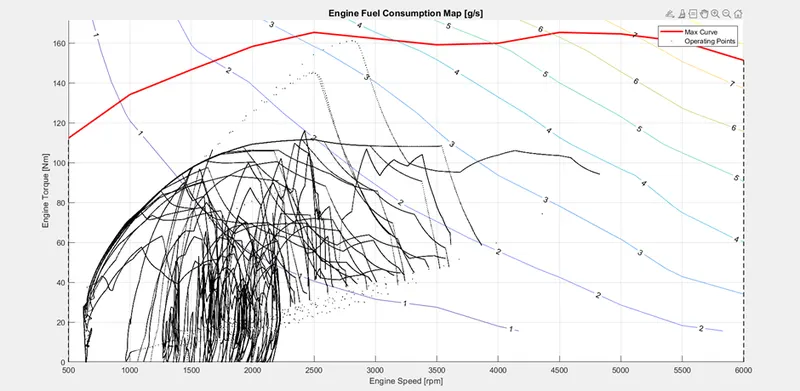
d. Plotting the engine operating points on the engine fuel map.

e. Plot motor speed, torque, and motor input power.

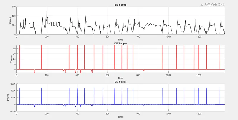
From the plots its seen that the torque is provided by the motor at lower speeds and during the stop and go situations also the torque in negative direction while braking and in the HWFET cycle we will observe that the motor torque use in minimal or mainly during the starting stage.

f. Plot pack voltage, current and SoC.

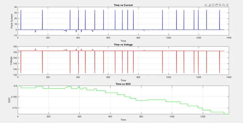
Since the torque is provided by the E motor the battery gets discharged and through SOC plot we can see that the battery is getting charged while regen braking.

g. Plot the motor operating points on the motor input power map, with the motor max motoring and generating torque curves.

The same set of plots for the HWFET drive cycle gives outputs as,

a. Time trace for engine, transmission input, transmission output and wheel speeds.

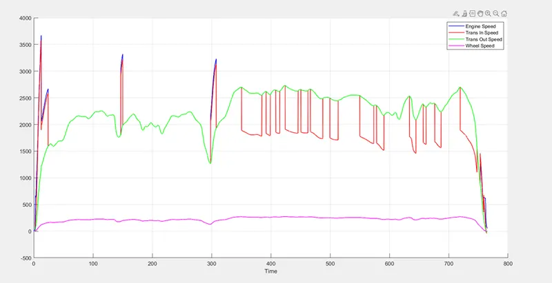
From the above figure we can see the loss occured while the engine speed is transmitted to wheels.

b. Plotting engine torque, engine power, fuel rate and fuel consumption.

c. Plotting accelerator and brake pedal, gear command, vehicle desired and actual speed, vehicle distance.

d. Plotting the engine operating points on the engine fuel map.

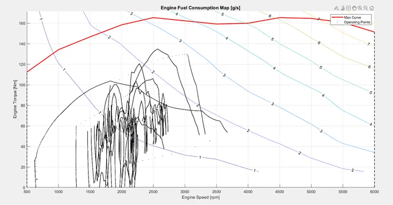
The engine operating points are plotted and its seen that all the operating points fall within the max torque curve.

e. Plot motor speed, torque, and motor input power.

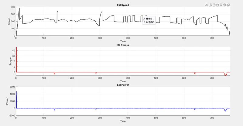
From the above figure we can see that the motor is only used during the initial period and only regen braking happens in later stages, whereas in UDDS the engine was used during the stop and go situations.

f. Plot pack voltage, current and SoC.

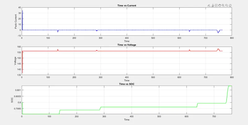
In this plot we can see that the controller uses the E motor in the initial period hence the SOC is decreases. And as the vehicle drive cycle is mainly in highways minimal braking is done and it almost runs in higher speeds so most of the time torque is provided by the engine and the battery is getting charged through regen braking.

g. Plot the motor operating points on the motor input power map, with the motor max motoring and generating torque curves.

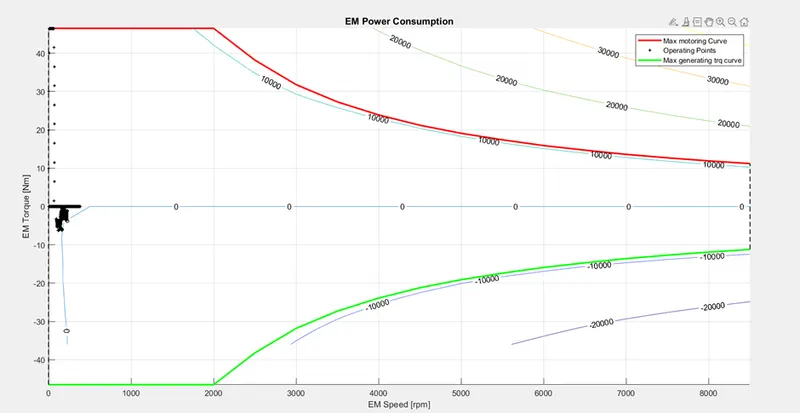
From the plot we can see that the motor operates at lower speeds only.

CONCLUSION:

The forward energy-based fuel consumption model of a P1 HYBRID vehicle is modelled using SIMULINK. And the required plots are plotted for both the mentioned drive cycles (i.e., UDDS and HWFET). The fuel economy for the respective cycles are mentioned below,
1. UDD : 14.773935 kmpl (for conventional vehicle 13.633082 kmpl)
2. HWFET : 16.966816 kmpl (for conventional vehicle 16.307528 kmpl)

We can clearly see there is a boost in fuel economy in both the cycles when compared with the conventional powertrain model. However, the boost is high in UDDS when compared with the HWFET as it involves more stop and go conditions thereby utilizing the E motor and battery pack more effectively.

From the plot of the engine, transmission in, transmission out and wheel speeds we can see that the engine produces the max speed and due to some losses the transmission in speed is reduced and due to transmission losses the transmission out speed is less than the in speed and finally due to the road load factor the wheel speed is very less when compared other speeds.
The gear vs time indicates the vehicle gear at that particular time period, and from the fuel flow rate, engine power and torque plot it is clearly visible that fuel flow rate increases as power and torque increases. In the plot of pedal % of accelerator and brake we can see when the brake is applied the spike of the brake curve increases and the same of accelerator pedal decreases.
In the plot of actual speed vs desired speed it is seen that our model traces the desired speed and the overshoot and under shoots are minimal.
And finally, the engine operating points are plotted on the engine fuel consumption map all the operating points fall below the max curve and within the range.
The E motor power and torque plots are also plotted by which it is observed when the E motor is working and also can see the state of charge increasing while braking.

References:

https://www.researchgate.net/publication/256202589_Comparative_analysis_of_forward-facing_models_vs_backward-facing_models_in_powertrain_component_sizing

https://skill-lync.com/student-projects/project-1-11612

https://x-engineer.org/mild-hybrid-electric-vehicles-mhev-types/