Rankine cycle Simulator
AIM:
To Create a Rankine Cycle Simulator using MATLAB, calculate the state points using the standard thermodynamic library XSteam and plot the H-S and T-S diagram.
THEORY:
The Rankine cycle is a vapor-powered cycle that describes the process by which heat engines, such as steam turbines, where mechanical work is extracted from a fluid as it moves between a heat source and heat sink. The Rankine cycle is an ideal cycle if water passes through the four components without pressure drops and irreversibility. The ideal Rankine cycle consists of the following four processes, as shown on the T-s diagram
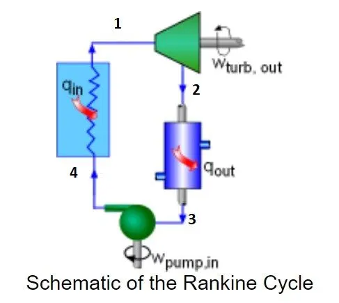
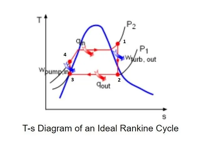
- 1-2: Isentropic expansion in a turbine
- 2-3: Constant pressure heat rejection in a condenser
- 3-4: Isentropic compression in a pump
- 4-1: Constant pressure heat addition in a boiler
(The sequence of processes may vary based on the numbering of state points in the T-S diagram, the sequence used here is to get the output in the desired form)
3-4: Isentropic compression in a pump
Water as a saturated liquid is compressed adiabatically from state 3 to state 4 by pumps. The liquid is pumped from the condenser to high-pressure boilers. In this process, the entropy remains unchanged, and pressure increases due to the compression of liquid. Work done by the pump is given by the change in enthalpy i.e., Wp= h4-h3.
4-1: Constant pressure heat addition in a boiler
This phase is also known as isobaric heat addition, there is a constant-pressure heat transfer to the liquid condensate from an external source. Water enters the boilers in compressed liquid state and leaves as a superheated vapor. Heat addition is given by Qin=h1-h4.
1-2: Isentropic expansion in a turbine
Superheated vapor/steam from the boiler expands adiabatically (the entropy remains unchanged i.e., S1=S2) from state 1 to state 2 in a steam turbine to produce work and then is discharged to the condenser. The steam works on the blades of the turbine and loses an amount of enthalpy equal to the work that leaves the system. The work done by the turbine is given by WT = h2 – h1.
2-3: Constant pressure heat rejection in a condenser
This phase is also known as isobaric heat rejection, the cycle completes by a constant-pressure process in which heat is rejected from the partially condensed steam. There is heat transfer from the vapor to cooling water flowing in a cooling circuit. The net heat rejected is given by Qout = h2 – h3.
Thermal efficiency of the Rankine cycle
The thermal efficiency of a Rankine cycle is given by the ratio of net work done to the heat input.
`eta = [W_[Net]]/[Q_[In]`
Where
`W_[Net]` is net work done i.e., `W_[Net] = W_T-W_P`
`Q_[In]` is heat input
OBJECTClVES OF THE PROJECT:
- Write a MATLAB code to simulate the Rankine cycle.
- To calculate the state points of the Rankine Cycle based on user inputs..
- To plot the corresponding T-S and H-S plots for the given set of inputs.
- To calculate the thermal efficiency of the Rankine cycle.
MAIN MATLAB PROGRAM
clear all
close all
clc

% Rankine cycle simulator
fprintf(' Rankine cycle Simulatorn');

% Displaying Rankine cycle process
fprintf('1-2 is the iscentropic expansion in the turbinesn');
fprintf('2-3 is constant pressure heat rejection by the condensern');
fprintf('3-4 is iscentropic compresssion in the pumpn');
fprintf('4-1 is constant pressure heat addition by the boilersnn');

% Defining the inputs
p1=input('Enter the pressure at the turbine inlet(in Bars): ');
t1=input('Enter the temperature at the turbine inlet (in Celcius): ');
p2=input('Enter the pressure at the condenser (in bars): ');

% Extracting enthalpy and entropy
h1=XSteam('h_pt',p1,t1); %Enthalpy
s1=XSteam('s_pt',p1,t1); %Entropy

% process 1-2
% Reversible adiabatic process, Entropy is constant
s2=s1;
sf2=XSteam('sL_P',p2);
sg2=XSteam('sV_P',p2);
hf2=XSteam('hL_P',p2);
hg2=XSteam('hV_P',p2);
hfg2=hg2-hf2;
sfg2=sg2-sf2;
x2=((s2-sf2)/(sfg2)); % x2 dryness fraction
h2=hf2+(x2.*(hfg2));

% at point 3
% pressure remains constant
p3=p2;
h3=XSteam('hL_P',p3);
s3=XSteam('sL_P',p3);
v3=XSteam('vL_P',p3);

% at point 4
% Entropy is constant
s4=s3;
p4=p1;

% pump work wp=h4-h3=v3(p1-p2)
wp=v3*(p1-p2)*100;
h4=wp+h3;

%work done by steam on turbine
wt=h1-h2;

% net work done
wnet=wt-wp;

% heat supplied
Q1=h1-h4;

% Efficiency of rankine cycle
eff=(wnet/Q1)*100;

% steam rate in kg/hr
steam_r=(3600/(wt-wp));

% temp at state 3

t3=XSteam('Tsat_P',p3);
t2=t3;
cp4=XSteam('Cp_ps',p4,s4);
cv4=XSteam('Cv_ps',p4,s4);
k=cp4/cv4;
t4=t3/((p3/p4)^((k-1)/k));

% Temperature enthalpy and entropy at liquid and vapour
t6=XSteam('Tsat_P',p1);
s5=XSteam('sL_P',p1);
s6=XSteam('sV_P',p1);
h5=XSteam('hL_p',p1);
h6=XSteam('hV_p',p1);
t5=t6;

% for plotting
T=linspace(1,400,1000);
for i=1:length(T)
    sf(i)=XSteam('sL_T',T(i));
    sg(i)=XSteam('sV_T',T(i));
    hf(i)=XSteam('hL_T',T(i));
    hg(i)=XSteam('hV_T',T(i));
end

% T-S diagram
figure(1)
hold on
plot(sf,T,'color','r','linewidth',3);
plot(sg,T,'color','r','linewidth',3);
plot([s1 s2],[t1 t2],'color','b','linewidth',1.5);
plot([s2 s3],[t2 t3],'color','b','linewidth',1.5);
plot([s3 s4],[t3 t4],'color','b','linewidth',1.5);
plot([s4 s5],[t4 t5],'color','b','linewidth',1.5);
plot([s5 s6],[t5 t6],'color','b','linewidth',1.5);

sc1=linspace(s6,s1,1000);
for k=1:length(sc1)
    Tc1(k)=XSteam('T_ps',p1,sc1(k));
end

plot(sc1,Tc1,'color','b','linewidth',1.5);
text(s1-0.1,t1+12,'1','fontsize',10);
text(s2,t2-5,'2','fontSize',10);
text(s3,t3,'3','horizontalalignment','right','verticalalignment','top','fontsize',10);
text(s4,t4,'4','horizontalalignment','right','verticalalignment','bottom','fontsize',10);
xlabel('Enthalpy [KJ/Kg]','fontsize',10)
ylabel('Temperature [Degree Celcius]','fontsize',10)
title('T-S diagram of rankine cycle','fontsize',12)

% for H-S diagram
figure(2)
hold on
plot(sf,hf,'color','r','linewidth',3);
plot(sg,hg,'color','r','linewidth',3);
plot([s1 s2],[h1 h2],'color','b','linewidth',1.5);
plot([s2 s3],[h2 h3],'color','b','linewidth',1.5);
plot([s3 s4],[h3 h4],'color','b','linewidth',1.5);
plot([s4 s5],[h4 h5],'color','b','linewidth',1.5);
plot([s5 s6],[h5 h6],'color','b','linewidth',1.5);

sc2=linspace(s6,s1,1000);
for n=1:length(sc2)
    hc1(n)=XSteam('h_ps',p1,sc2(n));
end
plot(sc2,hc1,'color','b','linewidth',1.5);
text(s1,h1+50,'1','fontsize',10);
text(s2,h2-50,'2','fontSize',10);
text(s3,h3,'3','horizontalalignment','right','verticalalignment','top','fontsize',10);
text(s4,h4,'4','horizontalalignment','right','verticalalignment','bottom','fontsize',10);
xlabel('Entropy [KJ/KgK]','fontsize',10)
ylabel('Enthalpy [KJ/Kg]','fontsize',10)
title('H-S diagram of rankine cycle','fontsize',12)

% for results to display
fprintf('nRESULTs:n')
fprintf('nAt state pt1:nP1 is : %5.3f BarnT1 is : %5.3f Degree CelciusnH1 is : %5.3f KJ/KgnS1 is : %5.3f KJ/KgKn',p1,t1,h1,s1)
fprintf('nAt state pt2:nP2 is : %5.3f BarnT2 is : %5.3f Degree CelciusnH2 is : %5.3f KJ/KgnS2 is : %5.3f KJ/KgKn',p2,t2,h2,s2)
fprintf('X2 is : %5.3fn',x2)
fprintf('nAt state pt3:nP3 is : %5.3f BarnT3 is : %5.3f Degree CelciusnH3 is : %5.3f KJ/KgnS3 is : %5.3f KJ/KgKn',p3,t3,h3,s3)
fprintf('nAt state pt4:nP4 is : %5.3f BarnT4 is : %5.3f Degree CelciusnH4 is : %5.3f KJ/KgnS4 is : %5.3f KJ/KgKn',p4,t4,h4,s4)
fprintf('nWork done by turbine(wt) is: %5.3f KJ/Kgn',wt)
fprintf('nWork done by pump(wp) is: %5.3f KJ/Kgn',wp)
fprintf('nNet work done is : %5.3f KJ/Kgn',wnet)
fprintf('nThermal efficiency : %5.3f % nn',eff)
fprintf('nnSteam rate is : %5.3f kg/hrn',steam_r)
The above written is the MATLAB code to simulate the Rankine cycle. Initially in the code we are describing the process of the Rankine cycle as mentioned above. In the further lines the pressure data and the temperature data at the inlet of Turbine and condenser are taken as inputs.
Once the pressure and temperature data are stotred in the code, the enthalpy and entropy from the XSteam library provided are extracted. Similarly, at all the state points the required datas are determined using the XSteam library.
The code ‘h3=XSteam('hL_P',p3)’ is an example for extracting the enthalpy data from the Xsteam, here in XSteam('hL_P’,’p3’) the term 'hL_P’ specifies the enthalpy at liquid stage for given pressure and the term ‘p3’ is the input. Similarly all the other data are extracted and stored with respective variable.
The equations above mentioned for Net work done, Heat added, Work done by turbine, Work done by pump and thermal efficiency are written in the code form.
In order to plot the T-S diagram the temperatures at all the points are determined with the input data. The saturation line is plotted by using the for loop lines in the code. Similar sort of codes are written to plot the H-S diagram as well.
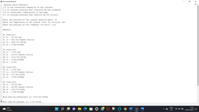
After plotting the required diagrams the outputs are displayed using the next set of commands, were all the state points data, thermal efficiency. Work done by pump, turbine and the heat inputs are displayed as output.
Below shown screenshot is of the output obtained on executing the code,
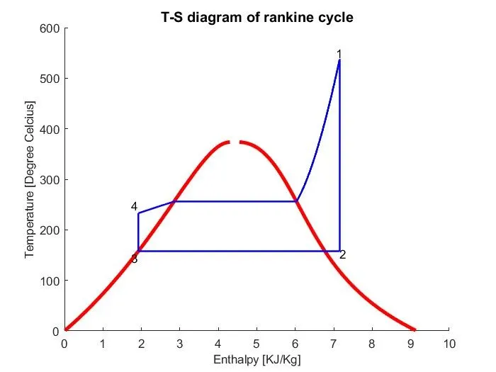
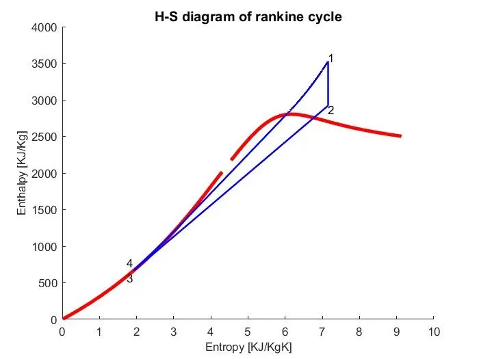
The output for the input,
Turbine Inlet temperature = 400° C
Turbine Inlet Pressure = 30 bars
Turbine Outlet Pressure = 0.05 bars = Condenser Inlet Pressure
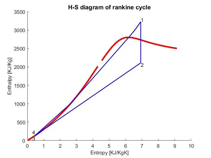
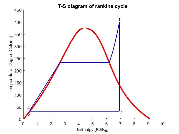
Screenshot of the command window,

CONCLUSlON:
- The code takes the inputs from the user and for the respective input the thermal properties are determined from XSteam.
- The T-S diagram and the H-S diagram are obtained after running the code.
- Rankine cycle is simulated where its processes are mentioned along with the state point data and other required outputs.
REFERENCE:
http://www.ecourses.ou.edu/cgi-bin/ebook.cgi?topic=th&chap_sec=10.1&page=theory
https://www.electrical4u.com/ideal-verses-actual-in-rankine-cycle/