Genetic Algorithm
AIM:
To write a MATLAB code to optimize the Stalagmite function using genetic algorithm and find the function’s global maxima. And also to plot the graph of F maximum v/s iterations for 3 different case studies.
THEORY:
Optimization is a process or methodology of making something such as a design, system, or decision as fully perfect, functional, or effective as possible. Optimization refers to finding the values of inputs in such a way that we get the best output values. It involves mathematical procedures such as finding the maximum/minimum of a function involved.
Global maximum is the greatest value among the overall elements of a set or values of a function whereas, Local maximum is the greatest element in the subset or a given range of a function. Similarly goes for the global minima and local minima, using the inbuilt function genetic algorithm (ga) in MATLAB we can determine the minimum of a function.
GENETIC ALGORITHM
A genetic algorithm is a method for solving both constrained and unconstrained optimization problems based on a natural selection process that mimics biological evolution. Genetic algorithms are a subset of a branch known as Evolutionary Computation.
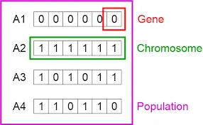
The population of individuals are maintained within the search space. Each individual is coded as a finite length vector of components. The algorithm randomly selects individuals from the current population and uses them as parents to produce children for the next generations. Over successive generations, the population evolves towards an Optimal solution. The below figure shows the stages of the genetic algorithm.

- Initialization of population
The process begins with a set of individuals called a population, each individual is a solution to a problem which we need to solve. An individual is characterized by set of parameters known as genes. Genes are joined into a string to form a chromosome. In a genetic algorithm, the set of genes of an individual is represented by using a string, in terms of alphabet. Chromosomes are often depicted by using binary values (strings of 0’s and 1’s).
- Fitness Function
The fitness function determines the ability of an individual to compete with other individuals. Then select the best ones to reproduce offsprings out of the available chromosomes, so each chromosome is given a fitness value. The probability that an individual will be selected for reproduction is based on the fitness value.
- Selection
The idea of selection is to select the fittest individuals and let the pass their genes to the next generation. Inspiration for this is survival of the fittest from the Darwin’s theory. GA tries to move the genotype to higher fitness in the search space. Too strong fitness can lead to sub optimal solutions and too weak fitness results in an unfocused search. Thus the fitness proportionate selection is used which is also known as roulette wheel selection, as a genetic operator used in genetic algorithms to select potentially useful recombination solutions.
- Reproduction
Generation of offsprings happens in two ways,
- Crossover
- Mutation
a. Crossover is a most significant phase of genetic algorithm, a random point is selected while mating a pair of parent to generate offsprings. Offsprings are created by exchanging the genes of parents until the crossover point is reached.
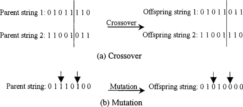
b. Mutation: in the new offsprings formed, some of their genes can be subjected to a low random probability mutation. This implies that some of the bits in the bot can be flipped. Mutation happens to take care of the diversity among the population and to stop premature convergence.
- Convergence
The algorithm terminates if the population has converged i.e., does not produce offsprings which are significantly different from the previous generation. Then it is said that the genetic algorithm has provided the optimal solution to the problem. Convergence happens when there is no improvement in the solution quality after completing a certain number of generations set beforehand, when a hard and fast range of generation is reached, or till an acceptable solution.
Governing Equations
The set of equation used in stalagmite function is shown in below image.
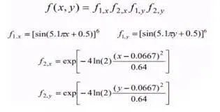
Syntax of GA
x = ga(fun,nvars,A,b,Aeq,beq,lb,ub,nonlcon,intcon,options)
fun = objective function (specified as a function handle or function name) which accepts row vector of length ‘nvars’ and return a scalar value.
Nvars = No. of variables (specified as a positive integer). The solver passes row vector of length ‘nvars’ to ‘fun’.
A & b = linear inequality constraints (specified as a real matrix). A is a matrix of order m*nvars where, ‘m’ is no of inequalities and b is a column matrix with ‘m’ elements.
Aeq & beq = Similarly as A and b Aeq and beq are for linear equalities.
Lb & ub = Lower bound (specified as real vector) and upper bound (`lb<=x<=ub`)
Nonlcon = Non-linear constraints (specified as a function handle or function name) is function that accepts a vector or array x and returns two arrays i.e., c(x) and ceq(x)
c(x) is an array of non-linear inequality constraints (`c(x)<=0`)
ceq(x) is an array of non-linear equality constraints (`c(x)=0`)
options = optimization options (specified as output of optimoptions or structure).
OBJECTClVES OF THE PROJECT:
- Write a MATLAB code to find the optimal solution for stalagmite function using genetic algorithm.
- Write the code for three different cases and plot graph of F maximum v/s No. of iterations.
STALAGMITE FUNCTION
% Stalagmite Function

function [F] = stalagmite(input_vector);

a = input_vector(1);
b = input_vector(2);

f1x = (sin(5.1*pi*a+0.5))^6;
f1y = (sin(5.1*pi*b+0.5))^6;

A = 4*log(2)*(a-0.0667)^2;
B = 4*log(2)*(b-0.0667)^2;

f2x = exp(-A/0.64);
f2y = exp(-B/0.64);

fxy = (f1x*f2x*f1y*f2y);

F = -fxy; % Inorder to get maximum value
end
The above written is the stalagmite function equation which is written in the form of MATLAB codes, in some cases variables ‘a’,’b’ and ‘A’,’B’ are used in order to simplify our code. Since GA is used to determine the minimum value and our objective is to find the maximum value the last line (F =-fxy) is added to get the maximum value.
MATLAB PROGRAM
clear all
close all
clc

% Defining our search space

x = linspace(0,0.6,150);
y = linspace(0,0.6,150);
iterations = 80; % No. of iterations to be performed

% Creating a 2-D array
[xx yy] = meshgrid(x,y);

% Evaluating the stalagmite function

for i=1:length(xx);
    for j=1:length(yy);
        input_vector(1) = xx(i,j);
        input_vector(2) = yy(i,j);
        f(i,j) = stalagmite(input_vector);
    end

end

% Study 1 Without boundary conditions

[inputs , fopt] = ga(@stalagmite,2)

tic
for i=1:iterations;
    [inputs fopt(i)] = ga(@stalagmite,2);
    xopt(i) = inputs(1);
    yopt(i) = inputs(2);
end
study1_time = toc

figure(1)
subplot(2,1,1)
hold on
surf(x,y,-f)

xlabel('x values')
ylabel('y values')
shading interp
plot3(xopt,yopt,-fopt,'marker','o','MarkerSize',5,'MarkerFaceColor','r')
title('Without boundary conditions')
subplot(2,1,2)

% To plot for F maximun v/s No. of iterations
plot(-fopt)

xlabel('no. of iterations')
ylabel('Function maximum')

% Study 2 With boundary conditions

tic
for i=1:iterations;
    [inputs fopt(i)] = ga(@stalagmite,2,[],[],[],[],[0;0],[0.6;0.6]);
    xopt(i) = inputs(1);
    yopt(i) = inputs(2);
end
study2_time = toc

figure(2)
subplot(2,1,1)
hold on
surf(x,y,-f)

xlabel('x values')
ylabel('y values')
shading interp
plot3(xopt,yopt,-fopt,'marker','o','MarkerSize',5,'MarkerFaceColor','r')
title('With boundary conditions')
subplot(2,1,2)

% To plot for F maximun v/s No. of iterations
plot(-fopt)

xlabel('no. of iterations')
ylabel('Function maximum')
inputs

% Study 3 With boundary conditions and increased polpulation

options = optimoptions('ga')
options =optimoptions(options,'PopulationSize',100)
tic
for i=1:iterations;
    [inputs fopt(i)] = ga(@stalagmite,2,[],[],[],[],[0;0],[0.6;0.6],[],[],options);
    xopt(i) = inputs(1);
    yopt(i) = inputs(2);
end
study3_time = toc

figure(3)
subplot(2,1,1)
hold on
surf(x,y,-f)
xlabel('x values')
ylabel('y values')
shading interp
plot3(xopt,yopt,-fopt,'marker','o','MarkerSize',5,'MarkerFaceColor','r')
title('With population 100')
subplot(2,1,2)

% To plot for F maximun v/s No. of iterations
plot(-fopt)

xlabel('no. of iterations')
ylabel('Function maximum')


% Study increasing the polulation from 100 to 300

options = optimoptions('ga')
options =optimoptions(options,'PopulationSize',300)
tic
for i=1:iterations;
    [inputs, fopt(i)] = ga(@stalagmite,2,[],[],[],[],[0;0],[0.6;0.6],[],[],options);
    xopt(i) = inputs(1);
    yopt(i) = inputs(2);
end
study4_time = toc

figure(4)
subplot(2,1,1)
hold on
surf(x,y,-f)
xlabel('x values')
ylabel('y values')
shading interp
plot3(xopt,yopt,-fopt,'marker','o','MarkerSize',5,'MarkerFaceColor','r')
title('With population 300')
subplot(2,1,2)

% To plot for F maximun v/s No. of iterations
plot(-fopt)

xlabel('no. of iterations')
ylabel('Function maximum')
Code Explanation
Initially, we are starting our code by clearing closing the previous memory using clear all close all and clc commands. Then we are specifying search space for our function using linspace command i.e., we are getting 150 values between 0 to 0.6 with same interval between them. Once get our one dimensional array of x and y using meshgrid command we are creating a 2-D array i.e. [xx, yy]. Now for loop is implemented inorder to run the stalagmite function for all the values of x and y. in this process 2 for loops are implemented one for the x values and the other for the y values. After the for loop ends the command of genetic algorithm is used i.e. ga(@stalagmite,2). Since we need a plot of Function maximum v/s No. of iterations again a for loop is implemented for the values from 1 to no of iteration to be performed. Here inorder to check the time taken by the algorithm to run is determined using ‘tic’ and ‘toc’ commands. Then the lines for plotting are written, the command subplot is used as we are getting two plots under one figure. In the first sub plot the line ‘surf(x,y,-f)’ plots the surface plot of (x,y,f) in the same plot we are plotting a 3-D plot of (xopt.yopt,fopt) using the line ’ plot3(xopt,yopt,-fopt,'marker','o','MarkerSize',5,'MarkerFaceColor','r')’. The next subplot is a plot of F maximum v/s No. of iterations.
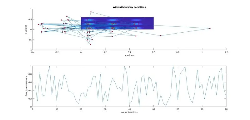
In our program, we are conducting 4 cases. In the first case the algorithm runs without boundary conditions the ga syntax is ‘ga(@stalagmite,2)’. The figure obtained while the 1st study is shown below
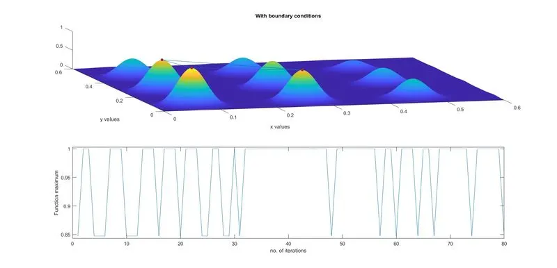
In the second study, we are specifying the boundary conditions now our ga syntax changes to ‘ga(@stalagmite,2,[],[],[],[],[0;0],[0.6;0.6])’ in this line A=[], b=[], Aeq=[] and beq=[] as no linear equalities does not exists. The lower limit is represented by [0;0] and upper limit is represented by [0.6;0.6]. The figure obtained while the 2nd study is shown below
In the 3rd and 4th study we are using optimoptions where we are specifying population size, so our code is modified by adding these lines ‘options = optimoptions('ga')
options =optimoptions(options,'PopulationSize',300)’
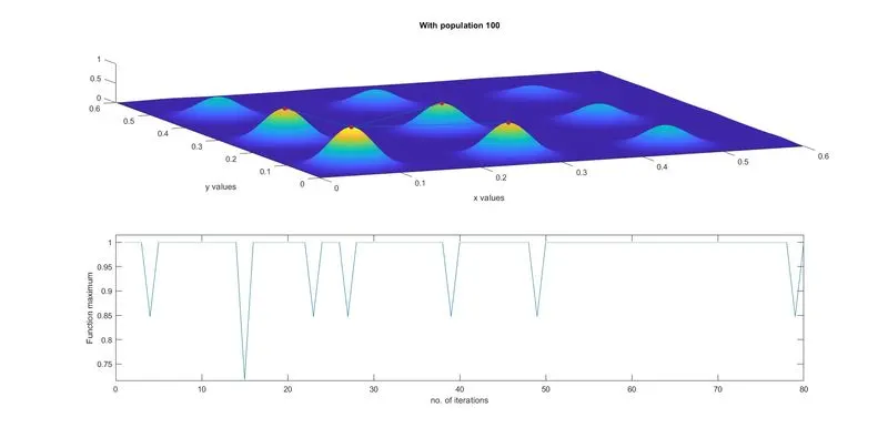
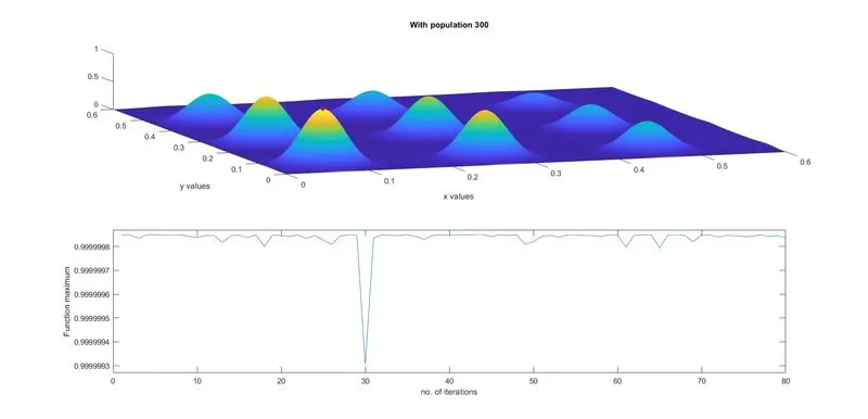
the syntax of ga changes to ‘ga(@stalagmite,2,[],[],[],[],[0;0],[0.6;0.6],[],[],options)’. The outputs of 3rd and 4th study is shown below
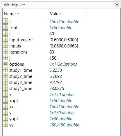
The final output image of the workspace is shown below
CONCLUSlON:
- The code is executed and the output plots are obtained, it was observed that the plot obtained each time was different however the values obtained were within the bounded limits.
- In study 1 it was observed that the plot was going outside the search space which was resolved in case 2 by specifying the boundary limits.
- The study time calculated for 3rd and 4th study was comparatively high this was because of specifying the individuals population which increases number of values thereby increasing the run time.
- It was observed that the more the number of population the closer we approached near our solution.
REFERENCE
https://www.tutorialspoint.com/genetic_algorithms/genetic_algorithms_introduction.htm
https://www.educba.com/what-is-genetic-algorithm/
https://www.geeksforgeeks.org/genetic-algorithms/
https://in.mathworks.com/help/gads/ga.html#mw_4a8bfdb9-7c4c-4302-8f47-d260b7a43e26