Week 3 - Solving second order ODEs

AIM:

To solve the Ordinary Differential Equation (ODE) using MATLAB program and using the output values obtained create an animation video of the motion of the pendulum.

THEORY:

Simple pendulum:

A simple pendulum has a heavy point mass (known as bob) suspended from a rigid support by a massless string. When the bob from its mean position is pulled to one side and then released, the pendulum is set to motion and the bob moves alternately on either side of its mean position.

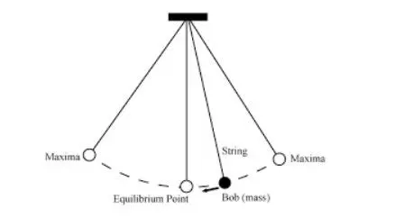
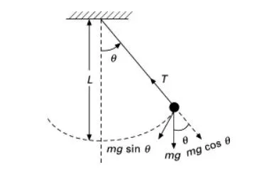
In the above fig ‘L’ is the length of the string/rod which is massless and ‘m’ is the mass of the bob. There are mainly two forces acting on the pendulum, the gravitational force acting downwards upon the bob and the tension force from the string that holds the bob. In addition to these forces there may be damping force due to friction at the pivot end or air resistance. At the end we will see how the angle `theta` of the pendulum varies as a function of time t.

The fig shows tangential and radial components of gravitational force on the pendulum bob. The radial component of the gravitational force gets balanced by the force exerted by the string, the only force producing the motion is the tangential component of the gravitational force. The damping force acts opposite to the direction of motion and is directly proportional to velocity. On considering all the forces we arrive at the Original Differential Equation (ODE). An ODE is an equality involving one or more functions and its derivatives.

`[d^2theta]/[dt^2]+b/m[d theta]/[dt]+g/Lsintheta`......................(1)

In order to write the MATLAB program, the 2^nd order ODE is broken down into series of 1^st order ODE and this transformation is shown below.

`theta = theta_1`

`[d theta]/dt=[d theta_1]/dt=theta_2`..............................(2)

`[d^2theta]/[dt^2] =[d[d theta_1]/dt]/dt= [d theta_2]/dt =-b/m[d theta]/[dt]-g/Lsintheta`.....................(3)

On substituting equations (1) & (2) in equation (3) we get,

`[d theta_2]/dt+b/m[d theta_1]/dt+g/Lsintheta_1`

or

`[d theta_2]/dt+b/mtheta_2+g/Lsintheta_1`

MATLAB PROGRAM

clear all
close all
clc

% inputs
b = input('Damping co efficient(b):');
g = 9.81;
l = input('Length of pendulum(L):');
m = input('Mass of pendulum(m):');

% initial condition
theta_0 = [0;3];

% time points
t_span = linspace(0,20,500);

% solve ODE
[t, results] = ode45(@(t,theta) ode_function(t,theta,b,g,l,m),t_span,theta_0);

figure(1)
% to plot displacement
plot(t,results(:,1))
hold on
% to plot velocity
plot(t, results(:,2))
ylabel('plot')
xlabel('time')

% plotting for animated video

ct = 1;
for i = 1:length(results(:,1))
        x_start = 0;
        y_start = 0;
        x_end = -1*sin(results(i,1));
        y_end = -1*cos(results(i,1));

        figure(2)
        plot([-1.5 1.5],[0 0],'linewidth',8,'color','b');
        hold on
         plot([x_start x_end],[y_start y_end],'linewidth',5,'color','g');
        hold on
        plot(x_end, y_end,'o','markersize',20,'markerfacecolor','r');
        hold off
  
        title('Pendulum motion');
        axis([-1.5 1.5 -1.5 0.5]);
        pause(0.03)

        M(ct)=getframe(gcf);
        ct=ct+1;

end

% To create an animated movie

movie(M)
videofile = VideoWriter('Simple pendulum.avi','Uncompressed AVI');
open(videofile);
writeVideo(videofile,M);
close(videofile);
    

The above written is MATLAB code to solve the ODE and to create an animated video of the motion of pendulum. Initially we are giving the inputs like damping coefficient, gravitational constant, length of the pendulum and mass of the pendulum. Here in these lines, we can give the inputs while writing the code i.e.,

Instead of the codes

b = input('Damping co efficient(b):');
g = 9.81;
l = input('Length of pendulum(L):');
m = input('Mass of pendulum(m):');

replacing by these codes

b = 0.05;
g = 9.81;
l = 1;
m = 1;

Once we run the program using the first set of codes, the command window asks for the inputs and inputs need to be entered in the command window.

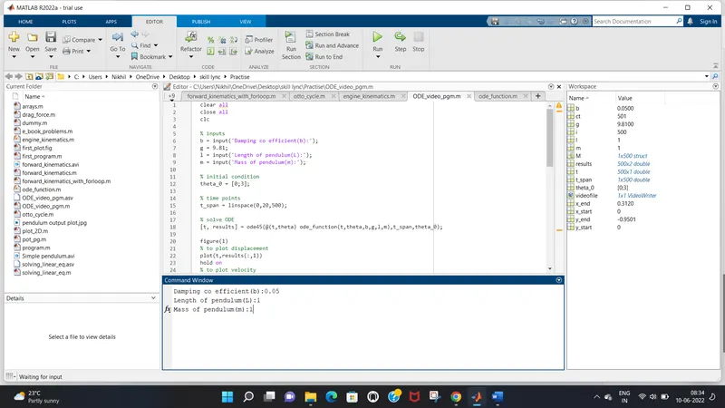
After giving the inputs we will specify the initial conditions i.e., angular displacement as 0 and angular velocity as 3. Then the time array is specified 500 values between 0 to 20 seconds are taken using command linspace(0,20,500).

In order to solve our ODE,

[t, results] = ode45(@(t,theta) ode_function(t,theta,b,g,l,m),t_span,theta_0);

The above line is written, here we are using ode45 code which is an inbuilt solver in MATLAB. The syntax for ode45 function is,

[tSol, ySol] = ode45(@ (t, y) function_name(t,y),[t0 tf],y0)

Where,

[tSol, ySol] = solution vector MATLAB returns ySol for each time tSol

Function_name = function that returns dy = F(t,y)

t0 y0 are initial condition representing y(t0) = y0

tf is the final value until which the solution is required

In our code the main inputs are (t, theta), the function name is ode_function, t_span as an array of time intervals and theta_0 as initial condition.

Now ode_function is a function written in a separate .m file shown below

function [dtheta_dt] = ode_function(t,theta,b,g,l,m)

theta1 = theta(1);
theta2 = theta(2);
dtheta1_dt = theta2;
dtheta2_dt = -(b/m)*theta2 -(g/l)*sin(theta1);
dtheta_dt = [dtheta1_dt; dtheta2_dt];

end

which breaks our 2^nd order ODE into 1^st order ODEs as shown in the above equations.

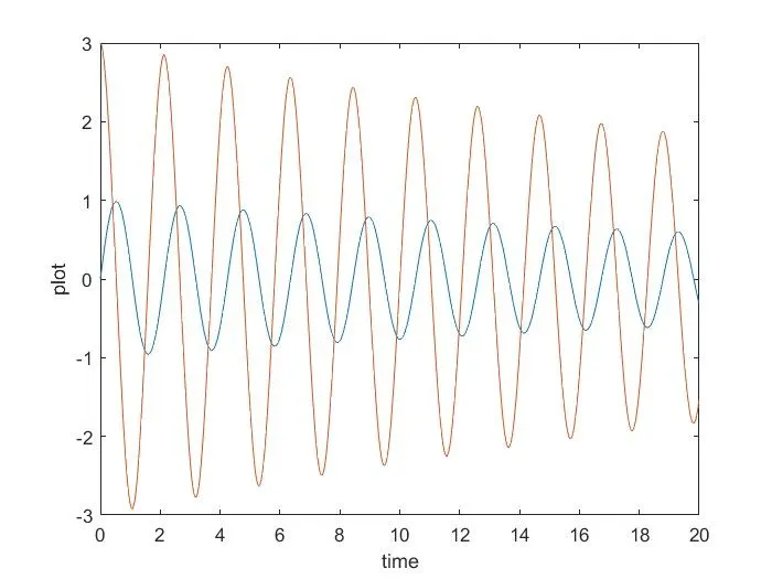
The next lines represent the codes to plot how angular displacement and angular velocity vary along with time.

plot(t,results(:,1))

plot(t,results(:,2))

The 1^st plot command plots the 1^st column(displacement) of the results matrix ((:,1) represents all the rows and 1^st column)and similarly 2^nd plot command for 2^nd column(velocity) of the result matrix.

The plot obtained by using these commands is shown below.

In order to cerate an animated video of the motion of the pendulum we will plot the positions of the pendulum for the respective angles made by the pendulum (i.e., theta). And then we will stitch all those plots together to create a movie.

We are using for loop to plot the displacement for all the time intervals. Since the string of the pendulum is a straight line and its initial point is fixed at the axis x_start and y_start is equal to 0. as theta is the displacement from the mean positions we get x_end = -1*sin(results(i,1)) and y_end = -1*cos(results(i,1)) (negative sign is in order to get the pendulum below the axis).

plot([-1.5 1.5],[0 0],'linewidth',8,'color','b') the plot of this line represents the fixed end of the pendulum.

plot([x_start x_end],[y_start y_end],'linewidth',5,'color','g') the plot of this line represents the string of the pendulum.

plot(x_end, y_end,'o','markersize',20,'markerfacecolor','r') this plot represents the bob of the pendulum.

As we are going to capture the plots for all the values of i in the for loop we will be using the command,

M(ct) = getframe(gcf)

Which captures the plots each time the for loop executed and stores it in an array M(ct) ct is contour which is initially defined as 1 before the for loop and at the end of the for loop it is incremented to ct = ct+1.

Once the for loops ends the remaining codes are executed where,

movie(M) command is given to create a movie in MATLAB, videofile = VideoWriter('Simple pendulum.avi','Uncompressed AVI') creates a .avi video file of name Simple Pendulum. After creating the file the command open(videofile) is executed to open the file and the command writeVideo(videofile,M) is to write the array of captured plots in that file and the finally the code close(videofile) is executed to close the video file.

The video link for the final output is mentioned below

https://youtu.be/f9hlJAOBRJU

CONCLUSION

Here are some figures for different values of damping coefficient

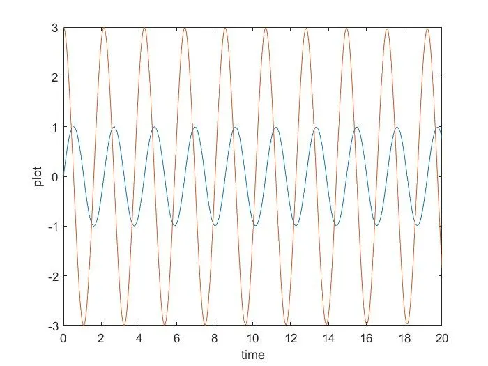
b=0

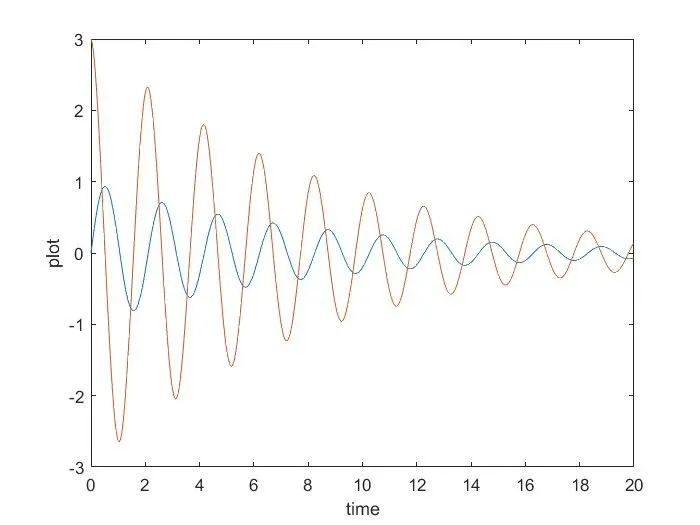
b=0.25

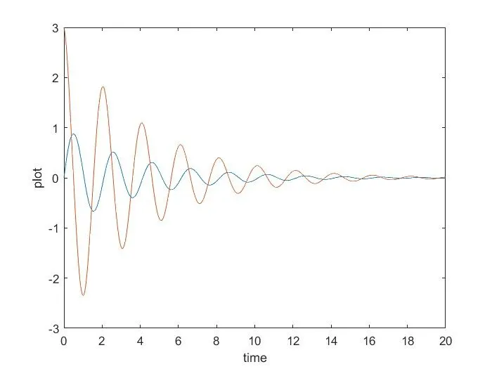
b=0.5

After seeing the results, it is found that the reduction of the amplitude in the plot is because of the damping factor.

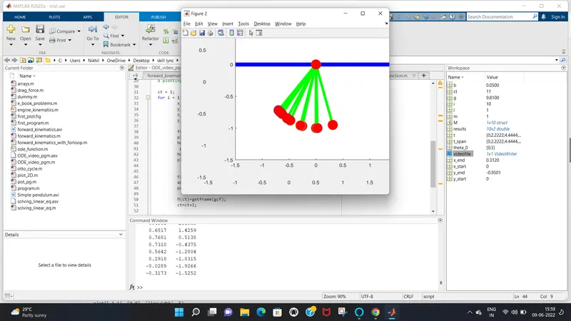
There were not any major errors thrown by MATLAB while programming the error found was while capturing the plots for animating the motion of pendulum is shown above. Which was sorted by using the code hold off in order to stop overlapping of previous plots.

REFERENCES

https://www.mathworks.com/videos/solving-odes-in-matlab-6-ode45-117537.html#:~:text=ODE45%20is%20usually%20the%20function,provide%20results%20at%20intermediate%20points.

https://services.math.duke.edu/education/ccp/materials/diffeq/pendulum/pend1.html

https://www.acs.psu.edu/drussell/Demos/Pendulum/Pendulum.html#:~:text=By%20applying%20Newton's%20secont%20law,enough%2C%20so%20the%20small%20angle