Project 1 - Data Handling and Interpolation

Project 1 :

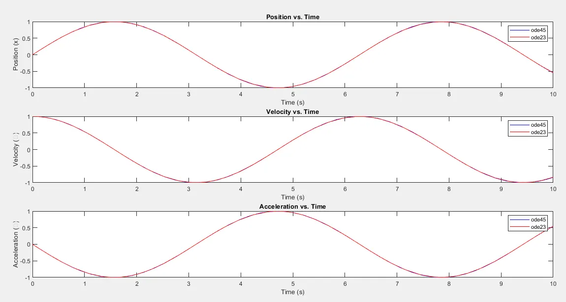
• Solve the simple harmonic oscillator equation [m . dx² / dt² = -k.x ] for a given m (mass) and k (spring constant) values using ‘ode45’ and ‘ode23’ solver in MATLAB.
• Plot x, x_dot (ẋ) & x_dot_dot (ẍ).
• Use the input dialog box to get ‘m’ & ‘k’ values from the user.
• Compare ‘ode45’ and ‘ode23’ plots and explain.

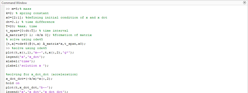
MATLAB CODE:

% Get user input for mass (m) and spring constant (k)
prompt = {'Enter mass (m):', 'Enter spring constant (k):'};
dlgtitle = 'Input';
dims = [1 35];
definput = {'1', '1'};
input = inputdlg(prompt, dlgtitle, dims, definput);

m = str2double(input{1});
k = str2double(input{2});

% Define the differential equation
fun = @(t, y) [y(2); -k / m * y(1)];

% Initial conditions: x(0) = 0, x_dot(0) = 1
y0 = [0; 1];

% Time span for the simulation
tspan = [0, 10];

% Solve using ode45 and ode23
[t45, sol45] = ode45(fun, tspan, y0);
[t23, sol23] = ode23(fun, tspan, y0);

% Extract the solutions
x45 = sol45(:, 1);
x_dot45 = sol45(:, 2);
x23 = sol23(:, 1);
x_dot23 = sol23(:, 2);

% Plot the results
figure;

% Position vs. Time
subplot(3, 1, 1);
plot(t45, x45, 'b', t23, x23, 'r');
xlabel('Time (s)');
ylabel('Position (x)');
legend('ode45', 'ode23');
title('Position vs. Time');

% Velocity vs. Time
subplot(3, 1, 2);
plot(t45, x_dot45, 'b', t23, x_dot23, 'r');
xlabel('Time (s)');
ylabel('Velocity (ẋ)');
legend('ode45', 'ode23');
title('Velocity vs. Time');

% Acceleration vs. Time
subplot(3, 1, 3);
x_dot_dot45 = -k / m * x45;
x_dot_dot23 = -k / m * x23;
plot(t45, x_dot_dot45, 'b', t23, x_dot_dot23, 'r');
xlabel('Time (s)');
ylabel('Acceleration (ẍ)');
legend('ode45', 'ode23');
title('Acceleration vs. Time');
end

M-SCRIPT

Result:

Project 2 :

Write a program to perform the following steps

• load altitude vs temperature data from the tables International Standard Atmosphere (ISA) ((click on the link))
• use the ‘polyfit’ function to determine a regression model: T = f(h) for the above table.
• evaluate the model determined using the ‘polyval’ function
• determine the goodness of fit (goodnessOfFit function)
• Generate comparative plot for the loaded and evaluated data
• store polyval evaluated data into a text file.

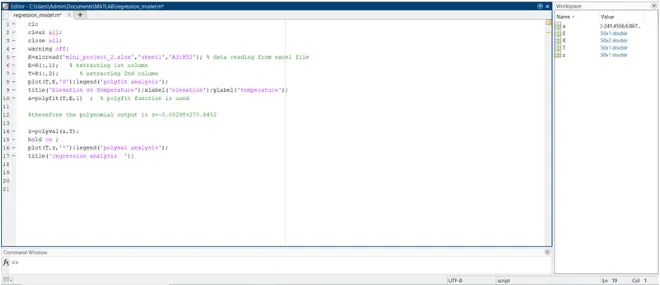
M-script:

warning off;
K=xlsread('mini_project_2.xlsx','sheet1','A3:B52'); % data reading from excel file
E=K(:,1); % extracting 1st column
T=K(:,2); % extracting 2nd column
plot(T,E,'O')
title('Elevation vs Temperature');xlabel('elevation');ylabel('temperature');
a=polyfit(T,E,1) % polyfit function is used for n=1(1st order )

%therefore the polynomial output is y=-0.0029x+270.6452

Project 3 :

Create a function to evaluate the following expression.

y= sin(x²) +cos(x) - 2 sin(x) cos(x)

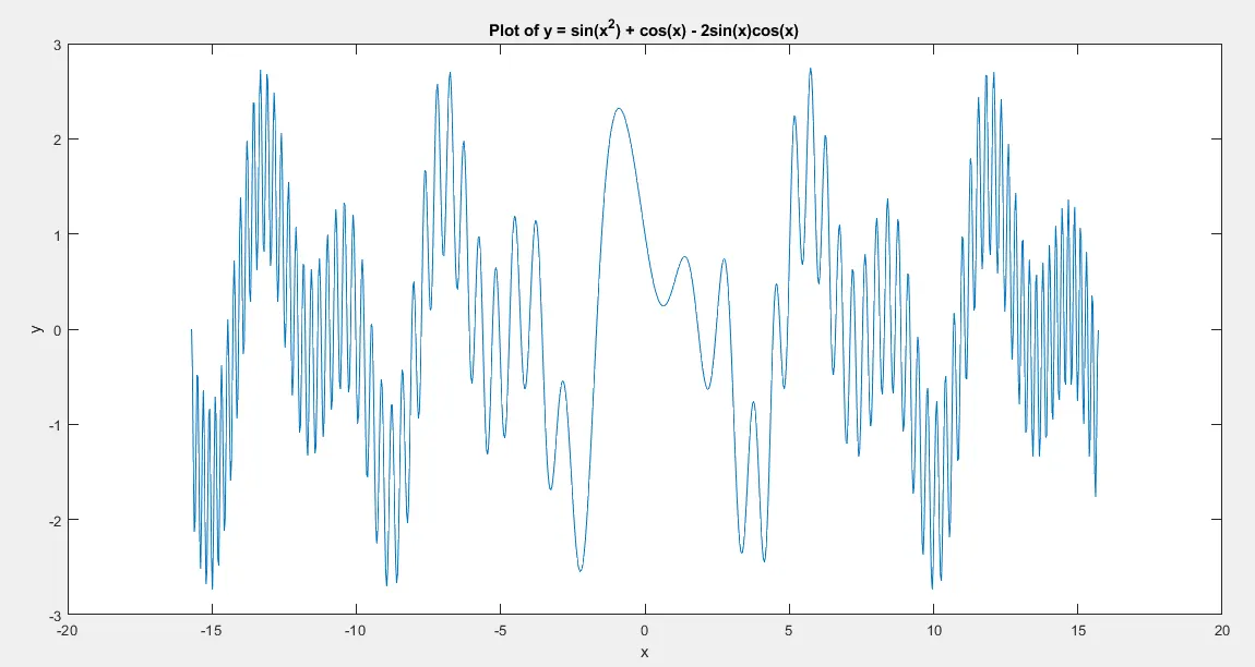
• Generate the plot and determine all local minima and global maxima values.
• Use the ‘gtext’ command to highlight the local minima and global maxima value in the graph.

Hint: make use of 'fminsearch' & 'max' commands.

sol:

M-script:

function find_extrema()
% Step 1: Create the function
f = @(x) sin(x.^2) + cos(x) - 2 * sin(x) .* cos(x);

% Step 2: Generate the plot of the function
x = linspace(-5*pi, 5*pi, 1000);
y = f(x);

figure;
plot(x, y);
xlabel('x');
ylabel('y');
title('Plot of y = sin(x^2) + cos(x) - 2sin(x)cos(x)');

% Step 3: Use 'fminsearch' to find local minima
local_minima_x = [];
local_minima_y = [];
for i = 1:length(x)-1
x0 = x(i);
x1 = x(i+1);
local_minima = fminsearch(f, [x0, x1]);
if local_minima(1) >= x(i) && local_minima(1) <= x(i+1)
local_minima_x(end+1) = local_minima(1);
local_minima_y(end+1) = f(local_minima(1));
end
end

% Step 4: Use 'max' to find the global maximum
[global_max_y, global_max_index] = max(y);
global_max_x = x(global_max_index);

% Step 5: Highlight the local minima and global maxima on the plot
hold on;
plot(local_minima_x, local_minima_y, 'ro', 'MarkerSize', 6, 'DisplayName', 'Local Minima');
plot(global_max_x, global_max_y, 'go', 'MarkerSize', 8, 'DisplayName', 'Global Maxima');
legend('Location', 'best');

% Add text labels near the points
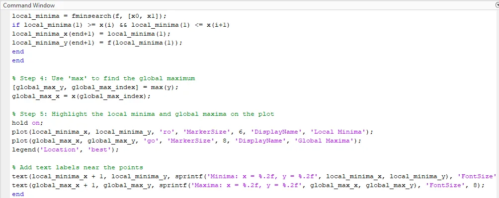
text(local_minima_x + 1, local_minima_y, sprintf('Minima: x = %.2f, y = %.2f', local_minima_x, local_minima_y), 'FontSize', 8);
text(global_max_x + 1, global_max_y, sprintf('Maxima: x = %.2f, y = %.2f', global_max_x, global_max_y), 'FontSize', 8);
end

RESULT:

Result:

Project 4 :

Give a brief note on the “contour” command. Illustrate with an example.

Note :

• For example, take simple code and execute in MATLAB.
• Attach the same along with the answer body.

The contour plot is formed by:

• Vertical axis: Independent variable 2
• Horizontal axis: Independent variable 1
• Lines: iso-response values, can be calculated with the help (x,y).

The independent variable usually restricted to a regular grid. The actual techniques for determining the correct iso-response values are rather complex and almost always computer-generated.

The contour plot is used to depict the change in Z values as compared to X and Y values. If the data (or function) do not form a regular grid, you typically need to perform a 2-D interpolation to form a regular grid.

For one variable data, a run sequence/ histogram is considered necessary. For two-variable data, a scatter plot is considered necessary. The contour plots can also polar co-ordinates (r,theta) instead of traditional rectangular (x, y, z) coordinates.

Types of Contour Plot:

• Rectangular Contour plot: A projection of 2D-plot in 2D-rectangular canvas. It is the most common form of the contour plot.
• Polar contour plot: Polar contour plot is plotted by using the polar coordinates r and theta. The response variable here is the collection of values generated while passing r and theta into the given function, where r is the distance from origin and theta is the angle from the positive x axis.
• Ternary contour plot: Ternary contour plot is used to represent the relationship between 3 explanatory variables and the response variable in the form of a filled triangle.

Contour plot can be plotted in different programming languages:

M-script:

x = -2:0.2:2;
y = -2:0.2:3;
[X,Y] = meshgrid(x,y);
Z = X.*exp(-X.^2-Y.^2);
contour(X,Y,Z,'ShowText','on')

• Matlab: functions such as contourf (2d-plot) and contour3 (3D-contour) can be used for contour plotting
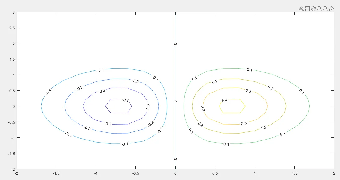
• RESULT:
•