Air standard - Otto cycle and its PV diagram using MATLAB
Q: Write a code that can solve an Otto cycle and make plots for it?
a) Create a PV diagram.
B) Output for thermal efficiency of the engine.
Ans: Otto cycle is a set of processes of a thermodynamic cycle, which explains about spark ignition piston engine. This cycle describes the changes that occur, like pressure, volume, temperature, entropy etc., during the process, when the mass of gas is considered. This cycle is commonly found in automobiles.
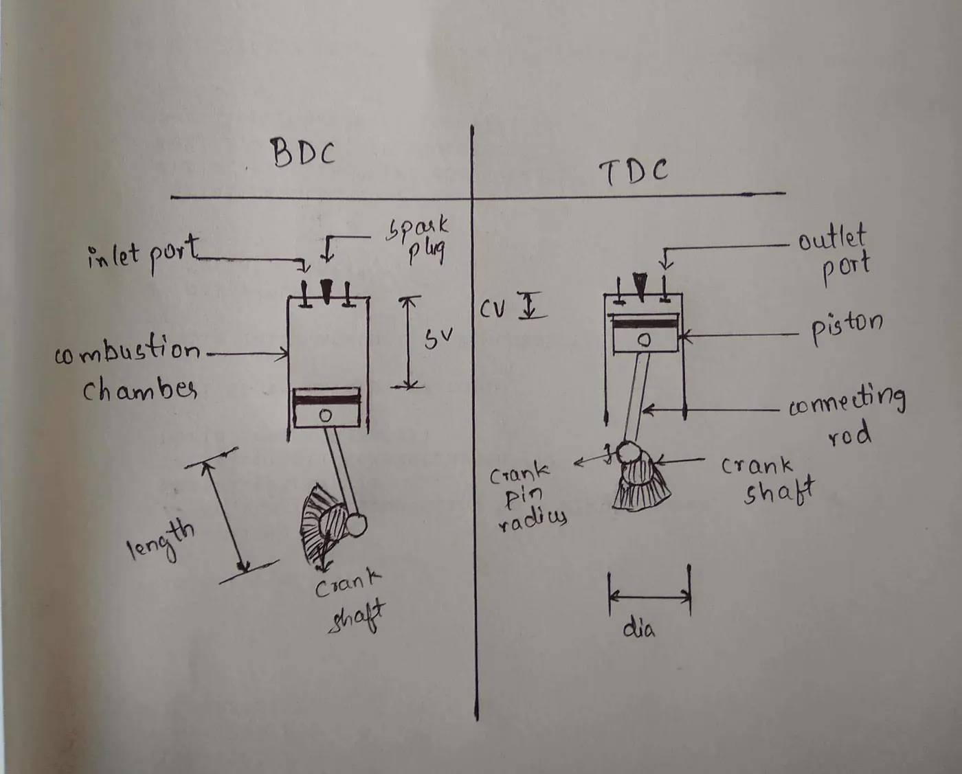
TDC: When the piston is at the top position of the cylinder known as TDC or Top Dead Centre.
BDC: When the piston is at the bottom position of the cylinder known as BDC or Bottom Dead Centre.
Engine parts and its position:
Otto cycle PV diagram:
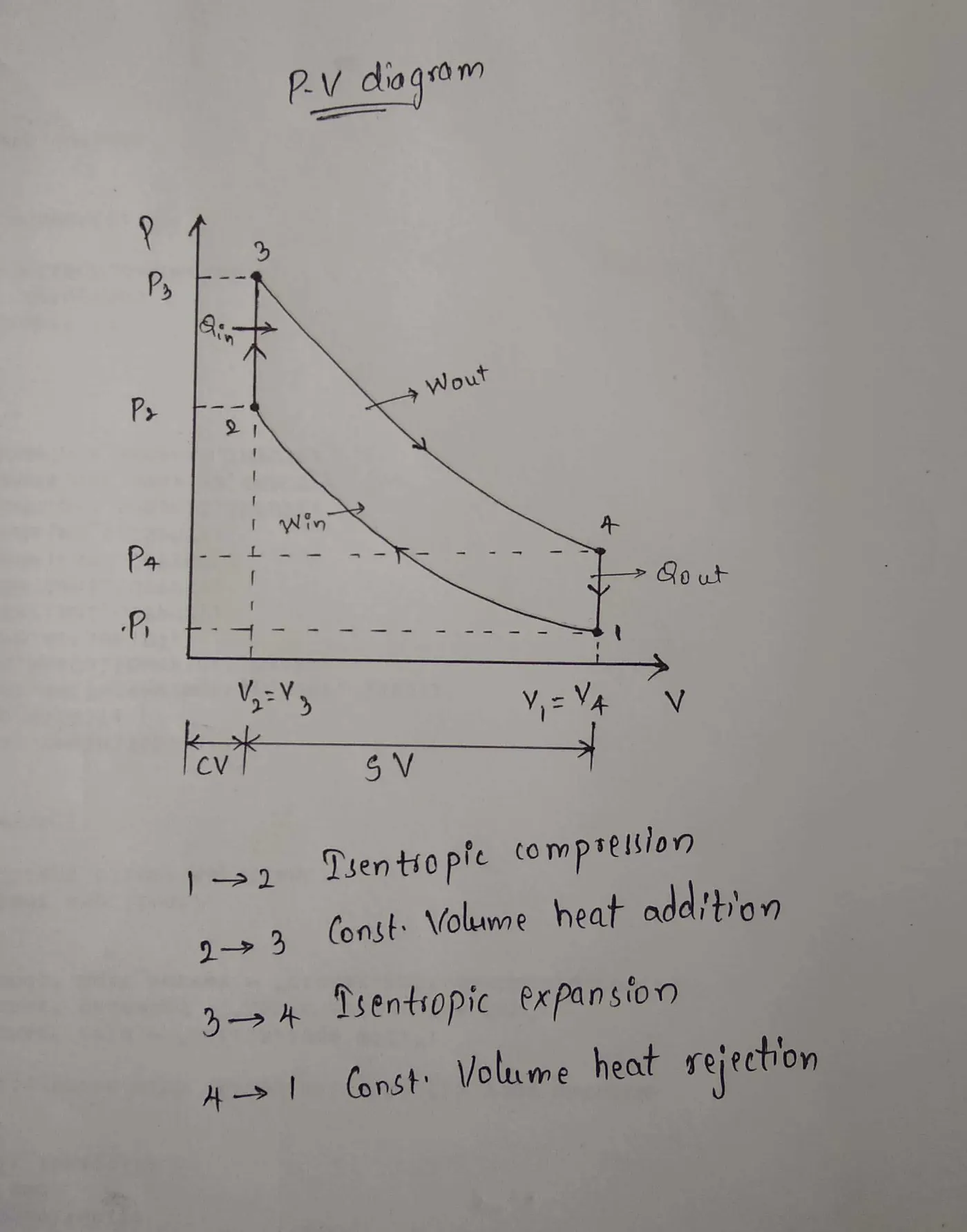
Otto cycle consists of 4 stages. They are:
- The Isentropic compression.
- The Isochoric process with heat addition.
- The Isentropic expansion.
- The isochoric process with heat rejection.
The Isentropic compression: This stage starts after suction of air-fuel mixture into the cylinder from the inlet port. Which means the piston is in BDC and contains the maximum volume. The piston is moved towards TDC and the compression takes place on the mixture. Here, the pressure is increased and the volume got decreased. Work is done on the system. This stage is also known as a compression stroke. This stage is represented by 1 to 2.
The isentropic compression ratio = V1/V2.
The Isochoric process with heat addition: When compression is done,(piston is at TDC) a spark is ignited to the mixture with the help of spark plug. The volume is constant and pressure is increased. This stage is also known as the ignition stage. This stage is represented by 2 to 3.
Explosion ratio = P3/P2.
The Isentropic expansion process: The piston is moved from TDC to BDC due to a force exerted by the mixture due to high pressure. Here, the work is done by the system. The volume is increased and the pressure is decreased. This is the stage where gases expansion occurs and known as the expansion process also a power stroke. This stage is represented by 3 to 4.
The isentropic expansion ratio = V1/V2.
The Isochoric process with heat rejection: The piston is at BDC and the pressure drops continuously with a constant volume. The gases will go out from the exhaust port, and the cycle comes to its initial stage. This stage is represented by 4 to 1.
Swept Volume: It is defined as the volume through which the piston is moved during a stroke.
Clearance Volume: It is defined as the volume left when the piston is at TDC.
Terms used in code:
- V1 = Volume at stage 1.
- P1 = Pressure at stage 1.
- T1 = Temperature at stage 1.
- V2 = Volume at stage 2.
- P2 = Pressure at stage 2.
- T2 = Temperature at stage 2.
- V3 = Volume at stage 3.
- P3 = Pressure at stage 3.
- T3 = Temperature at stage 3.
- V4 = Volume at stage 4.
- P4 = Pressure at stage 4.
- T4 = Temperature at stage 4.
- CR = Compression ratio.
- BD = Bore Diameter.
- SL = Stroke Length.
- CRL = Connecting rod length.
- SV = Swept Volume.
- CV = Clearance Volume.
- G = Gamma.
- TE = Thermal efficiency of an engine.
- SC = Starting crank angle.
- EC = Ending crank angle.
Here, we use both methods for solving this problem and finally we conclude, which is the correct solution for this problem.
Input values for code:
- G = 1.4
- P1 = 101325
- T1 = 500
- BD = 0.1
- SL = 0.1
- CRL = 0.15
- CR = 12
With these initial values, we can find other values by using different expressions in our code.
Formulas for finding values of other terms:
- SV = (pi /4) * B^2 * SL
- CV = SV/(CR - 1)
- V1 = SV + CV
- V2 = CV
- P2 = P1 * CR^G
- T2 = P2 * V2 * T1/(P1 * V1)
- P3 = P2 * T3/T2
- P4 = P3 * (V3/V4)^G
- TE = 1 - (1/(CR - 1)^G)
- TEP = TE * 100
Derivations at different state points:
- Variables at state point 1:
V1 = SV + CV ---------(formula 3)
P1 = 101325
T1 = 500 - Variables at state point 2:
V2 = CV --------(formula 4)
P2 * V2^γ = P1 * V1^γ (for isentropic expression)
⇒ P2 = P1 * (V1^γ/V2^γ)
⇒ P2 = P1 * (V1/V2)^γ
⇒ P2 = P1 * (CR)^γ (∵ V1/V2 = CR) --------(formula 5)
According to the ideal gas law
(P * V )/ T = Constant
⇒ (P1 * V1)/ T1 = (P2 * V2)/ T2
⇒ T2 = (P2 * V2 * T1)/(P1 * V1) --------(formula 6)
We know,
P * V^γ = constant
⇒ P1 * V1^γ = C
⇒ C = P1 * V1^γ - Variables at state point 3:
For constant volume process
V3 = V2
By ideal gas law
(P * V )/ T = Constant
⇒ (P2 * V2)/ T2 = (P3 * V3)/ T3
⇒ P3 = (P2 * V2 * T3)/(V3 * T2)
⇒ P3 = (P2 * V2 * T3)/(V2 * T2)
⇒ P3 = (P2 * T3)/(T2) --------(formula 7)
We can write,
P * V^γ = constant
⇒ P3 * V3^γ = C
⇒ C = P3 * V3^γ - Variables at state point 4:
For constant volume process
V4 = V1
We know,
P * V^γ = constant
⇒ P3 * V3^γ = P4 * V4^γ (for isentropic expression)
⇒ P4 = P3 * (V3^γ/V4^γ)
⇒ P4 = P3 * (V3/V4)^γ --------(formula 8)
Method 1:
Procedure:
- Write 'clear all', 'close all' and 'clc' statements.
clear all
close all
clc - Give input values and state variables as shown below.
G = 1.4
T3 = 2300
P1 = 101325
T1 = 500 - Give engine geometric parameters, such as bore diameter, stroke length, connecting rod length and compression ratio.
BD = 0.1
SL = 0.1
CRL = 0.15
CR = 12 - Calculating swept volume by using formula.
SV = (pi /4) * B^2 * SL - Calculating clearance volume by using formula.
CV = SV/(CR - 1) - Calculating volume V1 with the help of swept volume and clearance volume.
V1 = SV + CV - We know clearance volume is equal to V2 from the cycle since 2 to 3 is a constant volume process.
V2 = CV - Calculating state variables at state point 2.
P2 = P1 * CR^G
T2 = (P2 * V2 * T1)/(P1 * V1) - Calculating state variables at state point 3. We know that 2 to 3 is a constant volume process, then V3 equals to V2.
V3 = V2
P3 = (P2 * T3)/T2 - Calculating state variables at state point 4. We know 4 to 1 is a constant volume process, then V4 equals to V1.
V4 = V1
P4 = P3 * (V3/V4)^G - Calculating Thermal efficiency of an engine which is denoted by 'TE' and calculated by below formula.
TE = 1 - (1/(CR - 1)^G) - Then efficiency in percentage is given by
TEP = TE * 100 - Add statements for plotting a figure. Add 4 statements for plotting each point with a red colour.
figure(1)
plot(V1, P1, '*', 'color', 'r')
plot(V2, P2, '*', 'color', 'r')
plot(V3, P3, '*', 'color', 'r')
plot(V4, P4, '*', 'color', 'r') - Add labels for X-axis and Y-axis as Volume and Pressure respectively.
xlabel('Volume')
ylabel('Pressure')
Till now we get each point on cycle. Now we should join these points. - Add statement for joining points in another figure with cyan colour.
figure(2)
plot([V1 V2 V3 V4 V1], [P1 P2 P3 P4 P1], 'color', 'c') - Add labels for X-axis and Y-axis as Volume and Pressure respectively.
xlabel('Volume')
ylabel('Pressure') - We get the output with two plots and values in the command window. One plot consists of points represented by red dots and another plot consist of the cycle, where points are joined with lines.
Code:
clear all
close all
clc

% input
G = 1.4;
T3 = 2300;

% state variables

P1 = 101325;
T1 = 500;

% engine geometric parameters

BD = 0.1;
SL = 0.1;
CRL = 0.15;
CR = 12;

% calculating the swept volume and the clearance volume

SV = (pi/4) * BD^2 * SL ;

CV = SV/(CR - 1) ;

V1 = SV + CV ;
V2 = CV ;

% state variables at state point 2

P2 = P1 * CR ^G

T2 = P2 * V2 * T1 / (P1 * V1)


% state variables at state point 3

V3 = V2

P3 = P2 * (T3/T2)

% state variables at state point 4

V4 = V1

P4 = P3 * (V3/V4)^G

% Calculating thermal efficiency

TE = 1 - (1/(CR - 1)^G)

% Percentage

TEP = TE * 100

figure(1)
hold on
plot(V1, P1, '*', 'color','r')
plot(V2, P2, '*', 'color','r')
plot(V3, P3, '*', 'color','r')
plot(V4, P4, '*', 'color','r')
xlabel('Volume')
ylabel('Pressure')

figure(2)
plot([V1 V2 V3 V4 V1], [P1 P2 P3 P4 P1], 'color', 'c')
xlabel('Volume')
ylabel('Pressure')
Output in the command window:
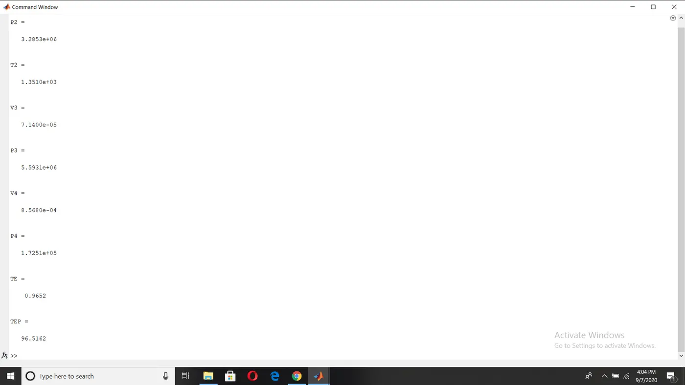
Output figures for method 1: We get two figures i.e., one with the lines which are points of pressure and volume in red colour and lines in cyan colour.
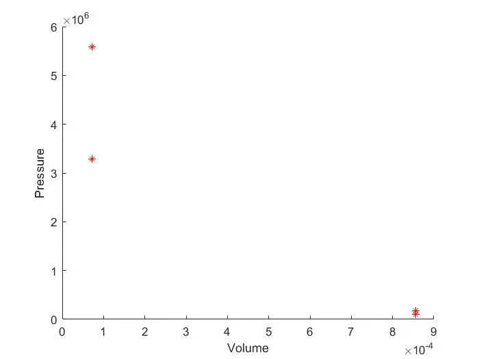
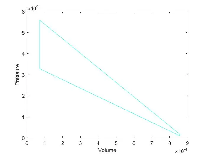
This output is incorrect because we know, both isentropic processes will not be in straight lines. Pressure and volume changes in a curve manner. We should correct these solutions by changing straight lines into curves. Only isochoric processes have straight lines. This can be done by method-2.
Method 2:
To solve volume changes that occur inside the combustion chamber the below expression is used. The expression is derived from piston kinematics. The relation is a non-dimensional of a slider-crank model. In this relation, we solve, with the help of a crank angle.
V/CV = 1 + 0.5(CR - 1)[R + 1 - cos(theta) - (R^2 - sin(theta)^2)^0.5]
Since it is a very large expression, we divide it into various terms.
term1 = 0.5(CR - 1)
term2 = R + 1 - cos(theta)
term3 = (R^2 - sin(theta)^2)^0.5
Taking these terms with 'V' as a subject. We can write the whole expression as follows.
V = (1 + term1 * (term2 - term3)) * CV
We get more variables for finding the values.
R = ratio of connecting rod to crankpin radius.
a = crankpin radius
Since crankpin radius is half of the stroke length. We can write a formula as below.
a = SL/2
R = CRL/a
These expressions are added at starting of the code.
Procedure for code 1:
- In this code, we are adding the piston kinematic expression for calculation. Instead of writing the whole code in a single script, we are assigning a function to this expression and calling it into code 2.
- Add function for all input values, which is given by mathematical relation 'y = f(x, z, w,...etc)'
V = oc_func2(BD, SL, CRL, CR, SC, EC) - Give formulas for crankpin radius and ratio of connecting rod to crankpin radius.
a = SL/2
R = CRL/a - Calculating swept volume and clearance value.
SV = (pi /4) * B^2 * SL
CV = SV/(CR - 1) - We know the crank angle range is in between starting crank angle and ending crank angle, i.e., SC and EC. We are giving 100 values in this range. To get this result we use 'linspace' command.
theta = linpsace(SC, EC, 100) - We divided kinematic expression into 3 terms and write these in our code.
term1 = 0.5(CR - 1)
term2 = R + 1 - cos(theta)
term3 = (R^2 - sin(theta).^2).^0.5 - For complete expression, we need to join these terms.
V = (1 + term1 * (term2 - term3)).* CV - We gave all formulas and values in our code for solving. Now, we need to end our code with 'end' statement.
end
Code 1:
function V = oc_func2(BD, SL, CRL, CR, SC, EC)

a = SL/2 ;
R = CRL/a;

SV = (pi/4) * BD^2 * SL ;
CV = SV /(CR - 1) ;


theta = linspace(SC, EC, 100);

term1 = 0.5 * (CR - 1);
term2 = R + 1 - cosd(theta);
term3 = (R^2 - sind(theta).^2).^0.5;

V = (1 + term1 * (term2 - term3)).* CV;

end
Procedure for code 2:
- Write 'clear all', 'close all' and 'clc' statements.
clear all
close all
clc - Give input values and state variables as shown below.
G = 1.4
T3 = 2300
P1 = 101325
T1 = 500 - Give engine geometric parameters, such as bore diameter, stroke length, connecting rod length and compression ratio.
BD = 0.1
SL = 0.1
CRL = 0.15
CR = 12 - Calculating swept volume by using formula.
SV = (pi /4) * B^2 * SL - Calculating clearance volume by using formula.
CV = SV/(CR - 1) - Calculating volume V1 with the help of swept volume and clearance volume.
V1 = SV + CV - We know clearance volume is equal to V2 from the cycle since 2 to 3 is a constant volume process.
V2 = CV - Calculating state variables at state point 2.
P2 = P1 * CR^G
T2 = (P2 * V2 * T1)/(P1 * V1) - Give the expression for constant 'C'.
C = P1 * V1 ^ G - To plot the values in the plot, we need to find the values for piston kinematic formula. This means we need to call the function from the above code as shown below.
VC = oc_func2(BD, SL, CRl, CR, 180,0) - We are calling values for starting crank angle and ending crank angle and remaining values are taken from the input values. Volume compression contains no.of values derived from another function 'oc_func'.
- Give the expression for pressure compression.
PC = C./ VC.^G - Now, give variables at state point3. We know 2 to 3 is a constant volume process. Hence V3 equals to V2.
V3 = V2
P3 = P2 * T3/T2
C = P3 * V3^G - Here we call the function once more for process 3 to 4, for different 'theta' values.
VE = oc_func2(BD, SL, CRL, CR, 0, 180)
PE = C./ VE.^G - Calculating state variables at state point 4. We know 4 to 1 is a constant volume process, then V4 equals to V1.
V4 = V1
P4 = P3 * (V3/V4)^G - Calculating Thermal efficiency of an engine which is denoted by 'TE' and calculated by below formula.
TE = 1 - (1/(CR - 1)^G) - Then efficiency in percentage is given by
TEP = TE * 100
- Add statements for plotting a figure. Add 4 statements for plotting each point with a red colour. Add plot statements for Volume compression, Pressure compression, Volume expansion and Pressure expansion. These plots should be done in a sequence, starting from stage 1 to 4. Let's denote compression process with 'Comp' and expansion process with 'Expan'.
figure(1)
plot(V1, P1, '*', 'color', 'r')
Comp = plot(VC, PC, 'color', 'blue')
plot(V2, P2, '*', 'color', 'r')
plot(V3, P3, '*', 'color', 'r')
Expan = plot(VE, PE, 'color', 'magenta')
plot(V4, P4, '*', 'color', 'r')
- Add statements for plotting a figure. Add 4 statements for plotting each point with a red colour. Add plot statements for Volume compression, Pressure compression, Volume expansion and Pressure expansion. These plots should be done in a sequence, starting from stage 1 to 4. Let's denote compression process with 'Comp' and expansion process with 'Expan'.
- Till now we get points at different stages and also curve in stage 1 to 2 and 3 to 4, i.e., for both isentropic processes. We need to plot lines for both constant volume processes. Let's denote them with Iso1 and Iso2.
Iso1 = plot([V2 V3],[P2 P3], 'color', 'green')
Iso2 = plot([V4 V1],[P4 P1], 'color', 'yellow') - Add labels for X-axis and Y-axis as Volume and Pressure respectively.
xlabel('Volume')
ylabel('Pressure')
Hence, we get the correct plot, for all stages. - To avoid confusion, we denote notations for each process by using 'legend' command. By using this command, we denote each coloured line in the figure.
legend([Comp,Iso1,Expan,Iso2], {'Isentropic compression','Isochoric process with heat addition','Isentropic expansion','Isochoric process with heat rejection'})
Code 2:
clear all
close all
clc

% input
G = 1.4;
T3 = 2300;

% state variables

P1 = 101325;
T1 = 500;

% engine geometric parameters

BD = 0.1;
SL = 0.1;
CRL = 0.15;
CR = 12;

% calculating the swept volume and the clearance volume

SV = (pi/4) * BD^2 * SL ;

CV = SV/(CR - 1) ;

V1 = SV + CV ;

V2 = CV ;

% state variables at state point 2

P2 = P1 * CR ^G

T2 = P2 * V2 * T1 / (P1 * V1)

C = P1 * V1^G;

VC = oc_func2(BD, SL, CRL, CR, 180, 0)

PC = C./ VC.^G;

% state variables at state point 3

V3 = V2

P3 = P2 * T3/T2

C = P3 * V3^G;

VE = oc_func2(BD, SL, CRL, CR, 0, 180)

PE = C./ VE.^G;

% state variables at state point 4

V4 =  V1

P4 = P3 * (V3/V4)^G

% Calculating thermal efficiency

TE = 1 - (1/(CR - 1)^G)

% Percentage

TEP = TE * 100

figure(1)
hold on
plot(V1, P1, '*', 'color','r')
Comp = plot(VC, PC, 'color', 'blue')
plot(V2, P2, '*', 'color','r')
plot(V3, P3, '*', 'color','r')
Expan = plot(VE, PE, 'color', 'magenta')
plot(V4, P4, '*', 'color','r')
Iso1 = plot([V2 V3], [P2 P3], 'color', 'green')
Iso2 = plot([V4 V1], [P4 P1], 'color', 'yellow')
xlabel('Volume')
ylabel('Pressure')

% adding legends
legend([Comp,Iso1,Expan,Iso2], {'Isentropic compression','Isochoric process with heat addition','Isentropic expansion','Isochoric process with heat rejection'})
Output in the command window:
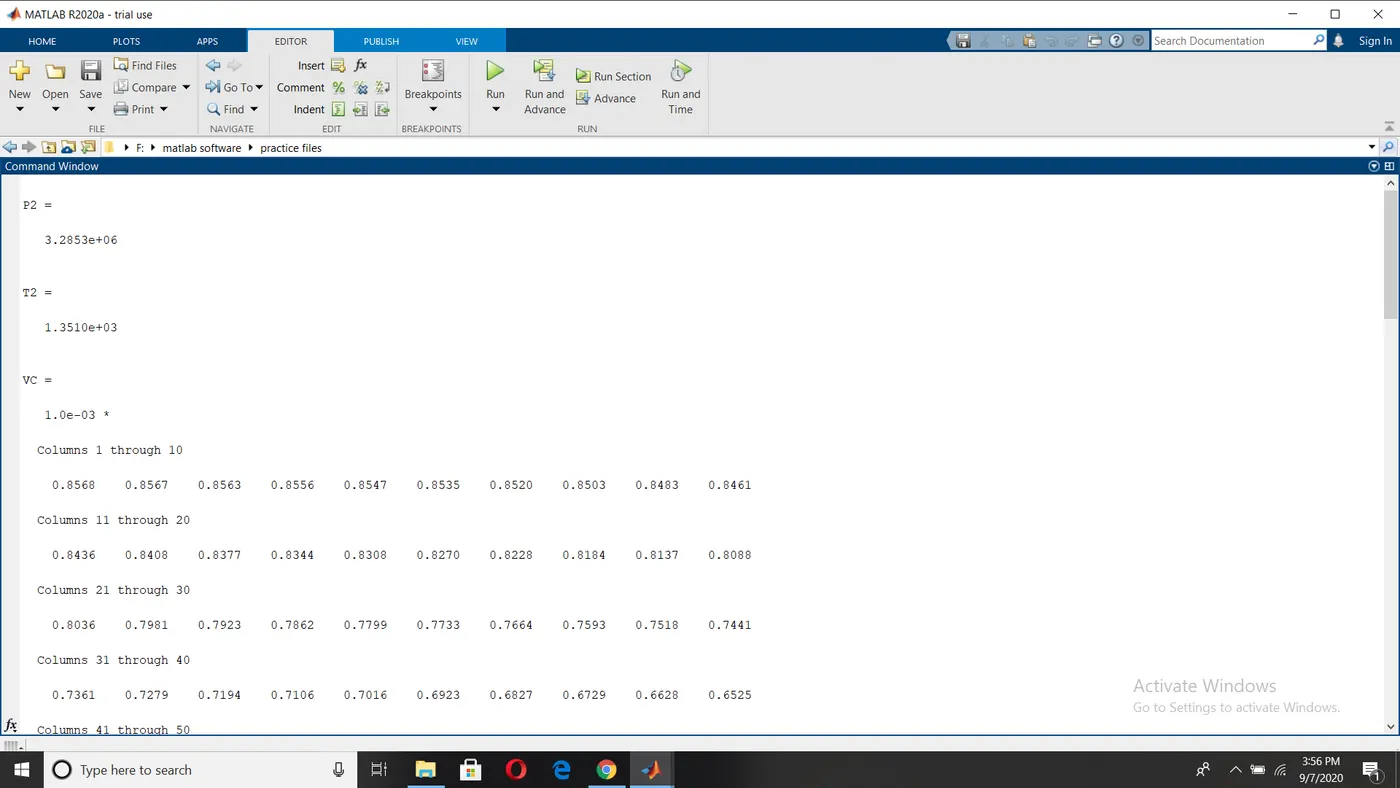
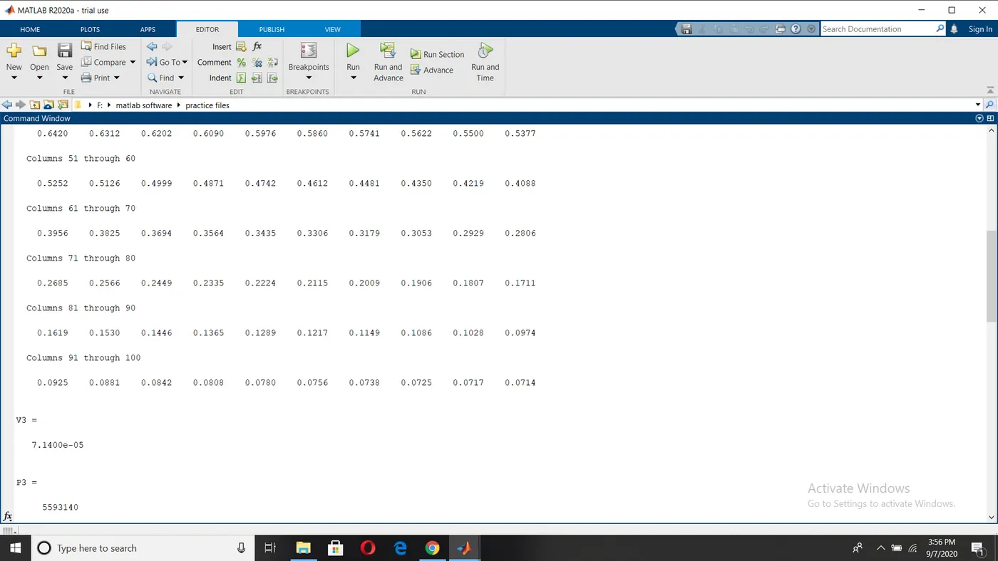
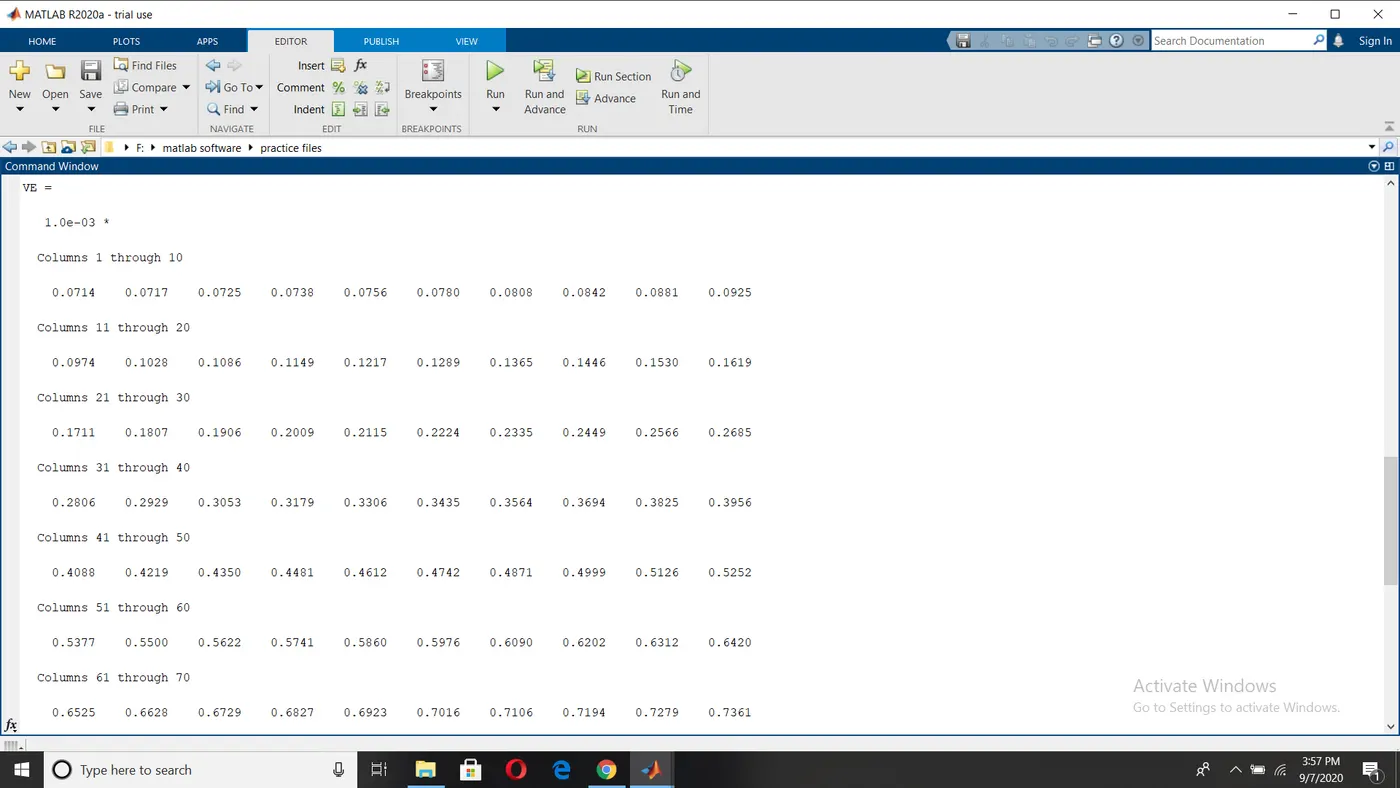
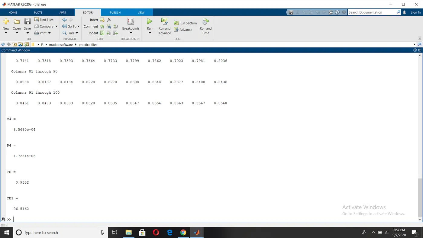
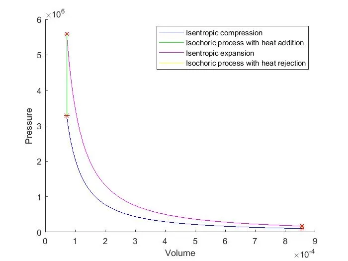
The final figure for this solution:
We get curves for both isentropic processes and straight lines for both isochoric processes. Points are also denoted by '*'. We can observe changes in volume and pressure and also constant volume.
Points to remember:
- Always remember, values of Pressure, Volume and Temperature are in Pascal, m^3 and Kelvin respectively.
- Length and diameter are in metres.
- Gamma and compression ratio doesn't have units.
- Add the element-wise operator whenever it is needed.
- Function name and filename should be the same.
- Function name and function calling should be the same.
- Both files should be in the same directory.
- Thermal efficiency is given in percentage.
- Always variables names should be given the same whenever required.
- 'r' letter indicated red colour and 'c' letter indicates cyan colour.
- Variables inside the function should be equal while giving values. No.of variables inside the function should be equal to no.of values while calling the function and also sequence should be the same.
- When angles are given in degrees 'cosd' and 'sind' is used. If they are in radians, use 'cos' and 'sin'.
- In the second method, we should execute the program for code 2 only. We don't get plot when we execute for code 1.
Errors:
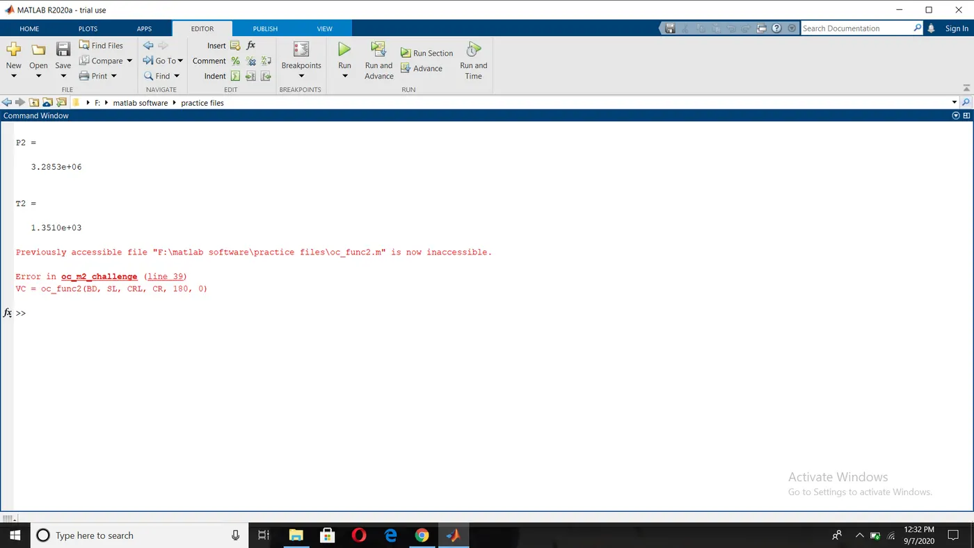
- When function file is saved or changed into another directory in the file manager, we get an error as shown below. To rectify this error, try to move the function file in the same directory where the main code file is present.
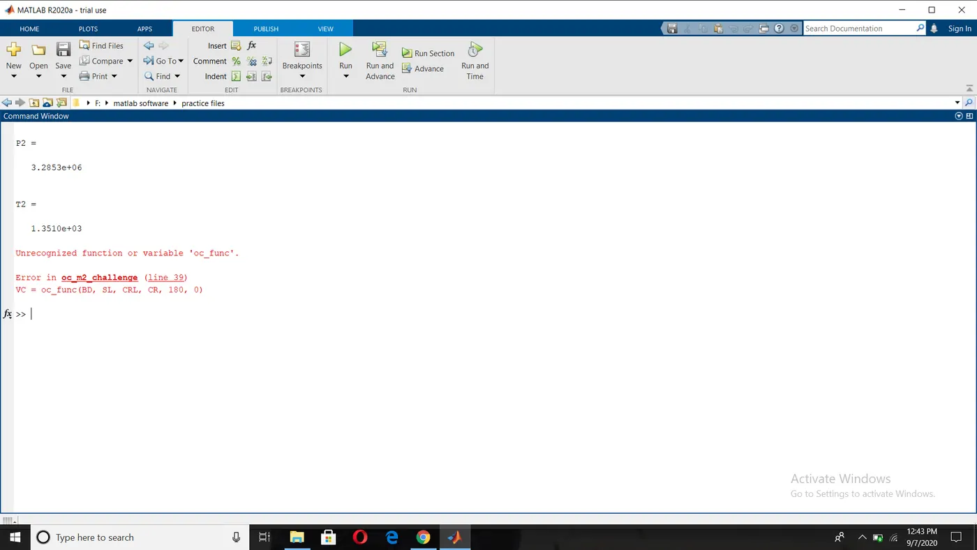
- When we write 'oc_func' instead of 'oc_func2', while calling function, it shows error in the command window as below. This can be rectified by checking, function name and function calling name.
Conclusion: Therefore, method 1 is incorrect and while plotting and solving isochoric processes. Method 2 is correct and the solution is given correctly and the plot is in curve manner as shown in the above figure.