WOT Condition

Aim:

1. To calculate the ratio of Hill-Climbing power required by fully loaded tata ultra truck to the half-loaded one.

2. To calculate the minimum length of the flyover.

3. To Prepare a new drive cycle excel file.

4. To Model the WOT (Wide Open Throttle) response of GM EV1 car.

Governing Equations:

• Hill-Climbing Power `(Phc):`

`Phc=Fhc⋅Vhc`

Where,

`Fhc=Hill` climbing Force``N`

`Vhc=Hill`climbing Velocity/speed (m/s)`

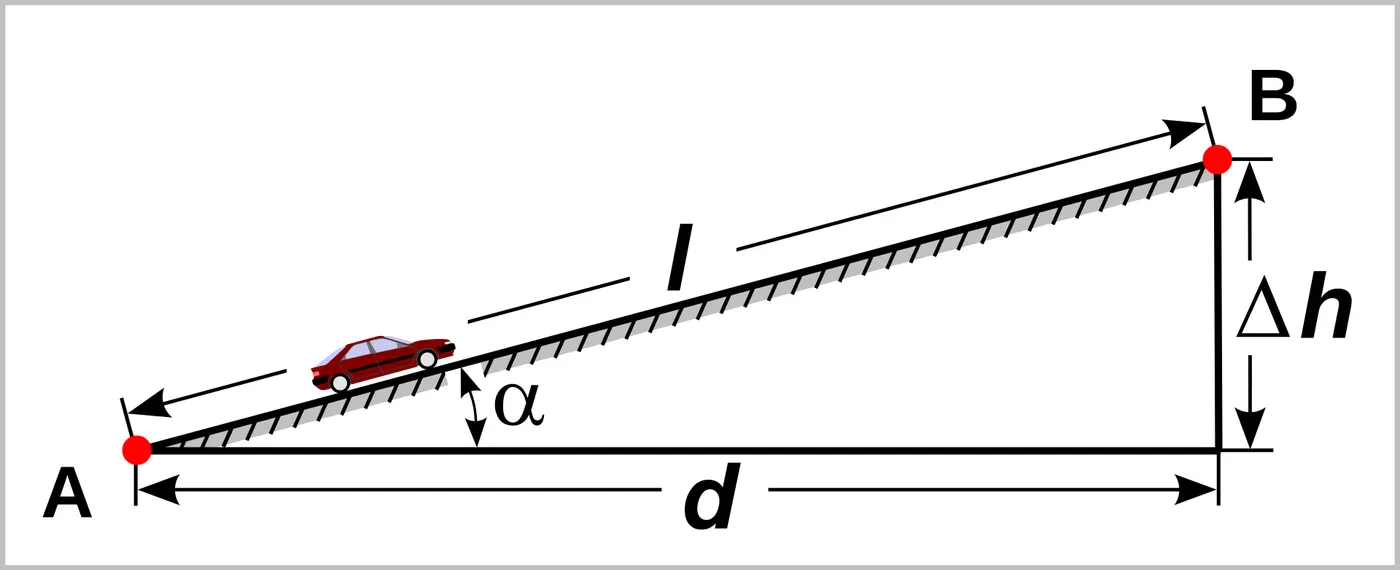
• Hill-Climbing Force `(Fhc):`

`Fhc=W⋅sin(θ)`

Where,

`W=Weight(kg)`

`θ=`Angle of Inclination`

• Gradeability`(G):`

`G=((Fte)/W-μrr)`

Where,

`Fte= Traction`Force``(N)`

`murr=` Coefficient of Rolling Resistance

• Inclination Angle `(θ):`

`θ=1/tan(G)`

Solution:

1. calculating the ratio of Hill-Climbing power required by "fully loaded tata ultra truck" to the "half-loaded one":

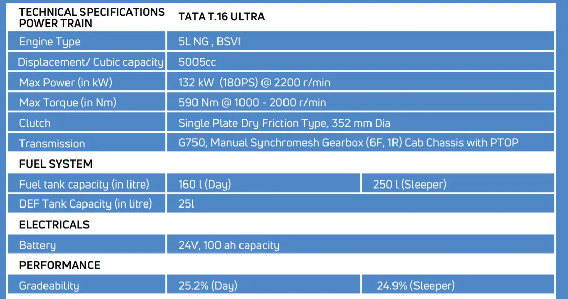
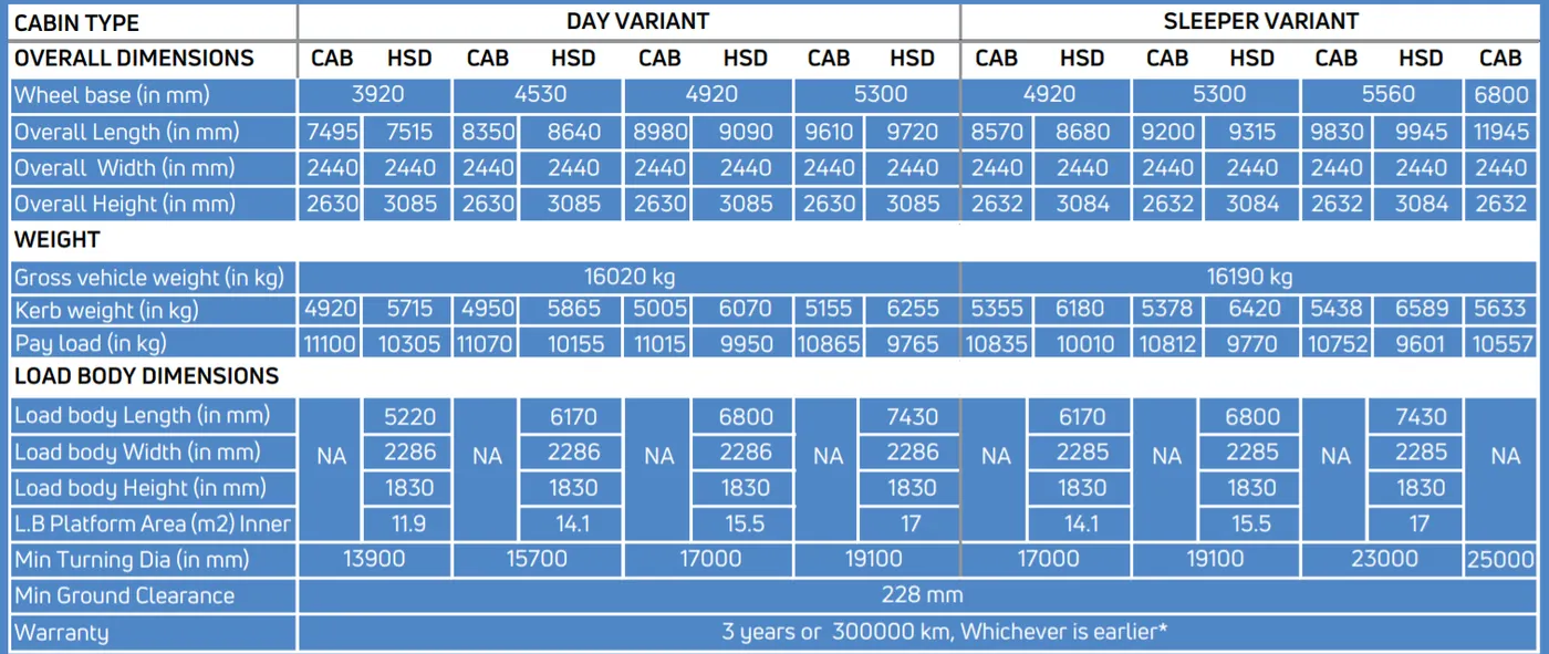
For the Calculation I have selected "TATA T.16 ULTRA".

• Hill-Climbimg power for fully-loaded Truck:

Selected - "Day variant"

Kerb weight = 4920 kg

Pay load = 11100 kg

Total Weight (W) = 16020 kg

Hill Climbing Speed (Vhc) = 30 kmph = 8.3 m/s

Gradeability (G) = 25.2%

Angle of Inclination `(θ) = 1/tan(G)= 14 Degrees`

Hill-Climbing Force `(Fhc1):`

`Fhc1=W⋅sin(θ)`

`=16020⋅sin(14)`

`= 15.869(kN)`

Hill-Climbing Power `(Phc1):`

`Phc1=Fhc⋅Vhc`

`=15.869⋅8.3`

`=131.7 kW`

• Hill-Climbimg power for half-loaded Truck:

Kerb weight = 4920 kg

Pay load = 11100/2 = 5550 kg

Total Weight (W) = 10470 kg

Hill-Climbing Force `(Fhc2):`

`Fhc2=W⋅sin(θ)`

`=10470⋅sin(14)`

`= 10.37kN`

Hill-Climbing Power `(Phc2):`

`Phc2=Fhc⋅Vhc`

`=10.37⋅8.3`

`=86kW`

Ratio of Hill-Climbing power required by "fully loaded tata ultra truck" to the "half-loaded:

`= (Phc1)/(Phc2)`

`=``137.786`

`= 1.6`

The ratio is `1.6`

2. Calculating the length of the flyover:

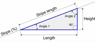
Summit height `(H)=5.5m`

Angle of inclination `(θ)=14Degrees`

`sin(θ)=H/L`

`sin(14)=5.5/L`

`L= 5.5/sin(14)`

`=22.7m`

L= length of flyover on one side.

There fore, the total mimimum length of the flyover is `=2L= 45.4m`

3.1. Preparing a new drive cycle excel file:

Drive Cycle File:

• https://drive.google.com/file/d/1r39vyC1Fu4IdipbQwQl7DXITRop0YC1B/view?usp=sharing

Procedure:

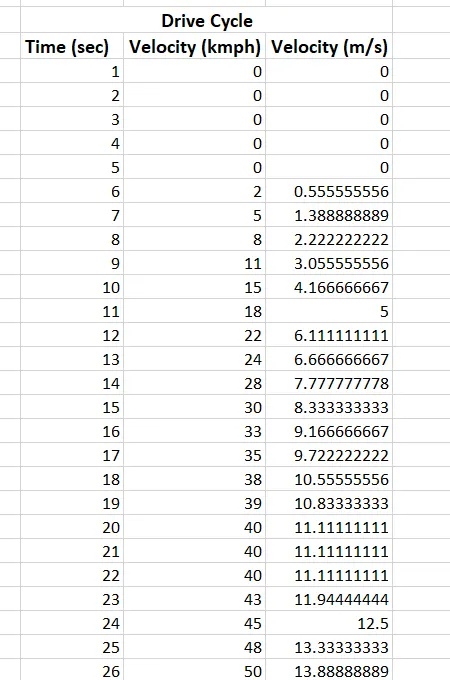
• Prepare a Drive Cycle in the Excel for 120 sec & velocity in (m/s) and copy the file to MATLAB current working path.
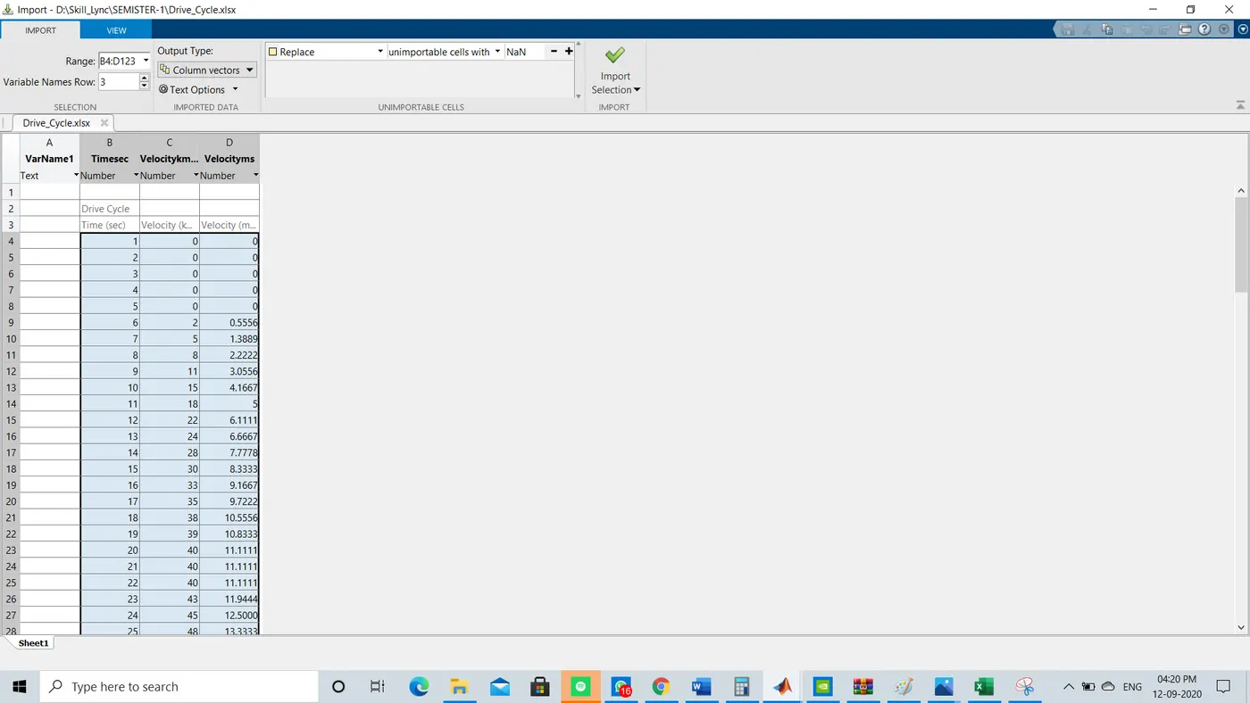
• Open the Excel file in the MATLAB and import the data of Time and velocity to workspace.
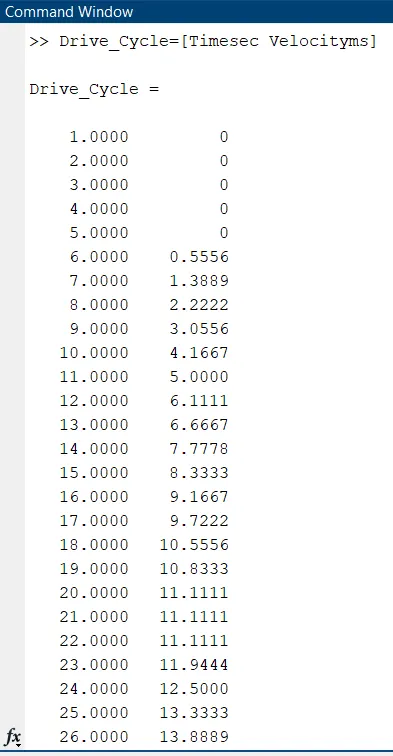
• Next, Define "Drive_cycle" as an array of Time & velocity.

• Excel sheet:

• Importing the data to the MATLAB

Output:

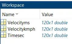
• Workspace & command window of Drive cycle.

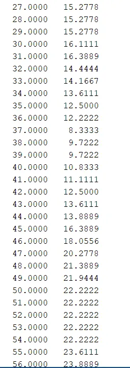
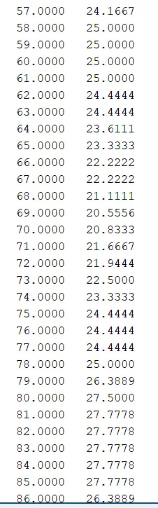
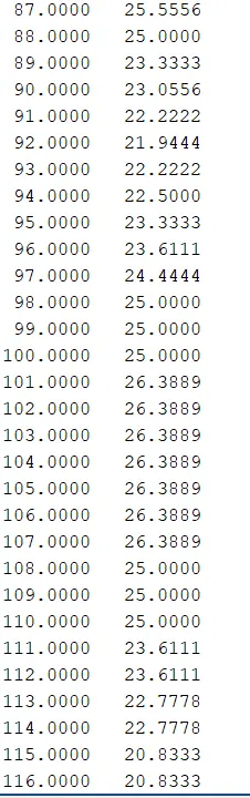
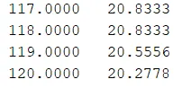
3.2. Driver Glider

Procedure:

• Download the VehicleModeling file and extarct and add to the current path in MATLAB.
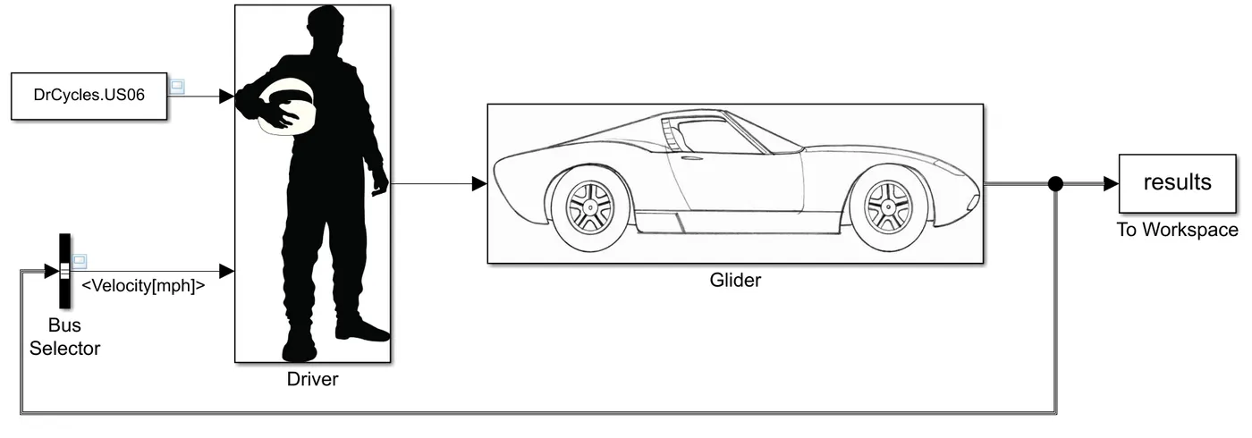
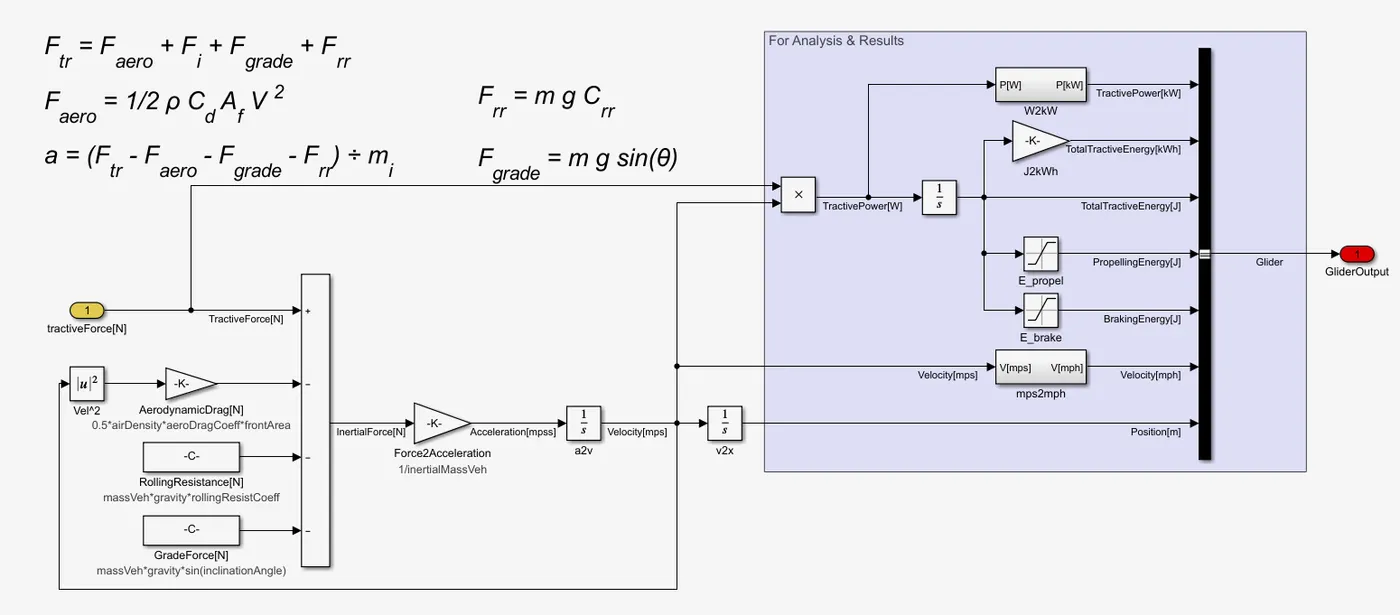
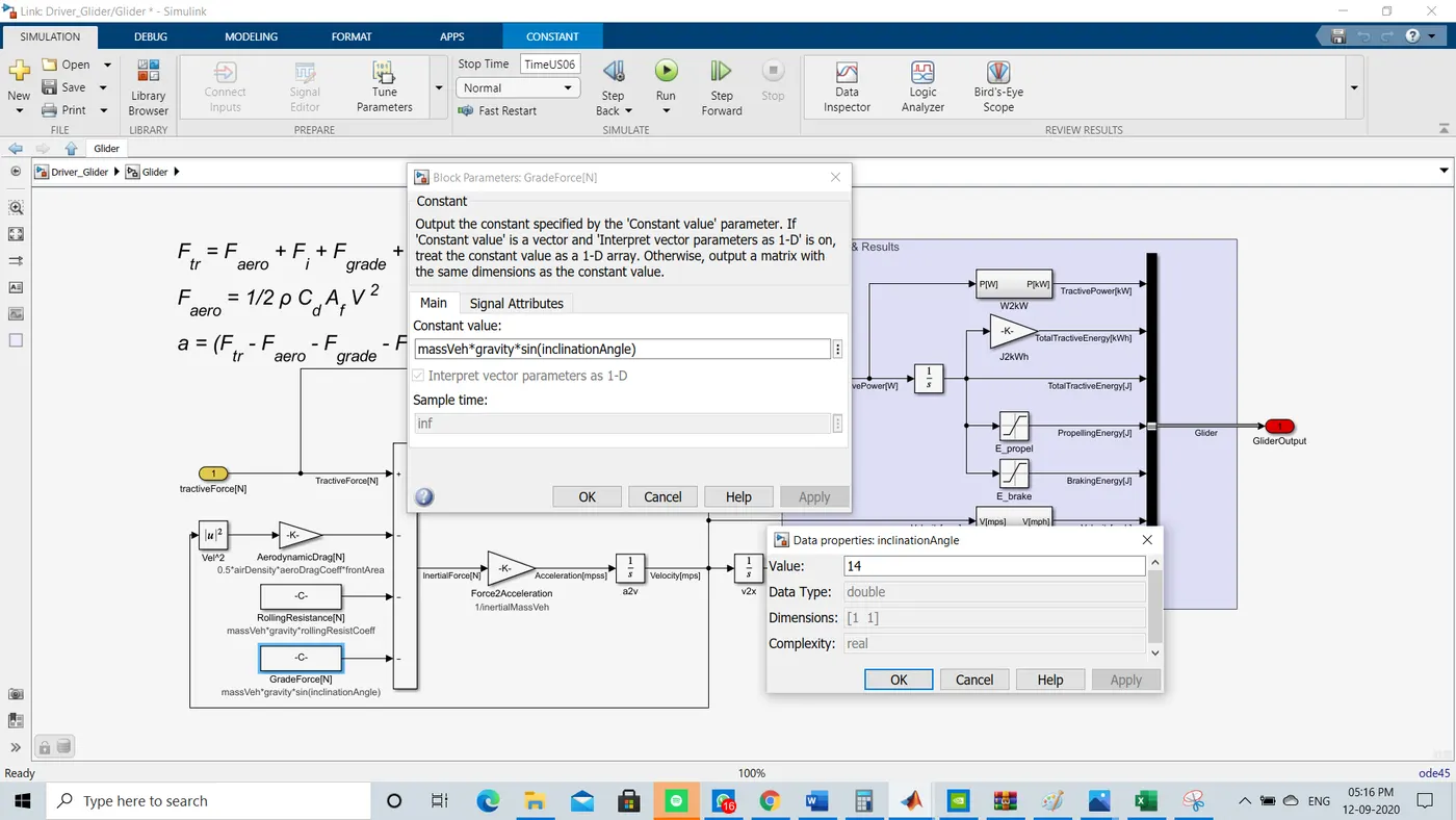
• Open the Drive_Glider.slx simulink and changed the angle of inclination to 14 Degrees and run the simulation.
• Observe the plot Time vs Velocity before and after changing the angle of inclination.
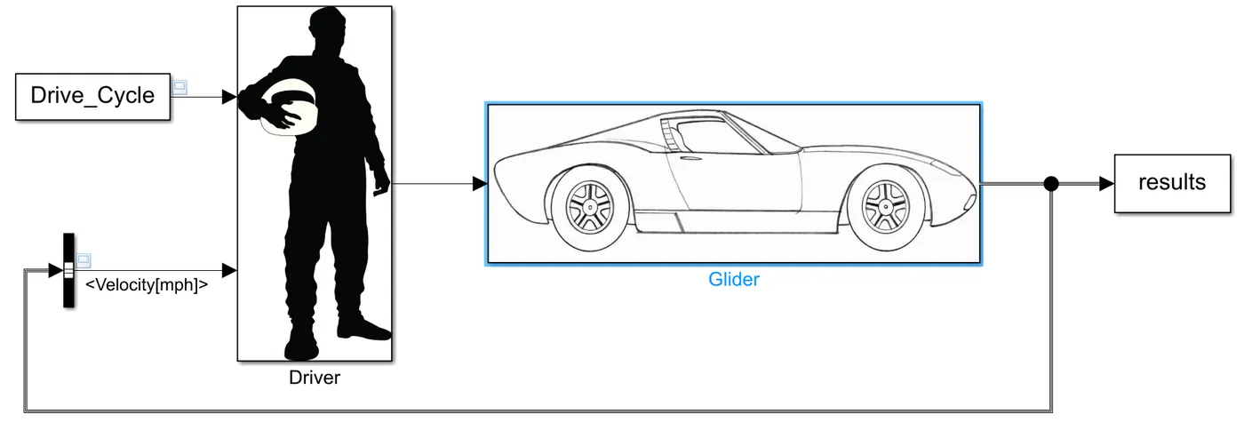
• Next, add the imported Drive cycle data of Time and Velocity in the block parameter.
• Run the simulation and compare the drive cycle plot with original Driver Glider.

• Original Driver Glider:

• Glider Subsystem

• After adding the imported Drive cycle data:

OutPut:

Results:

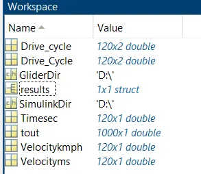
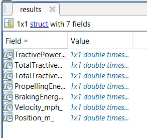
• Before adding imported drive cycle data

- Plot - Time vs Velocity for NO Inclination.

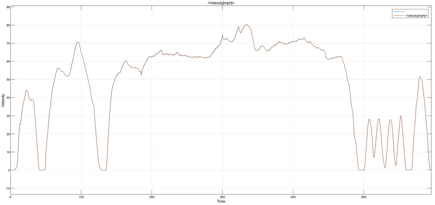
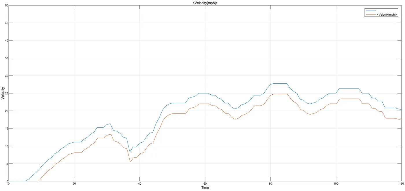
- Plot Time vs Velocity for 14Degrees Angle of Inclination.

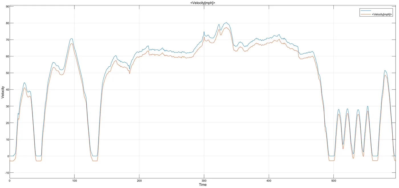
• After Adding imported drive cycle data:

- Plot - Time vs Velocity for NO Inclination.

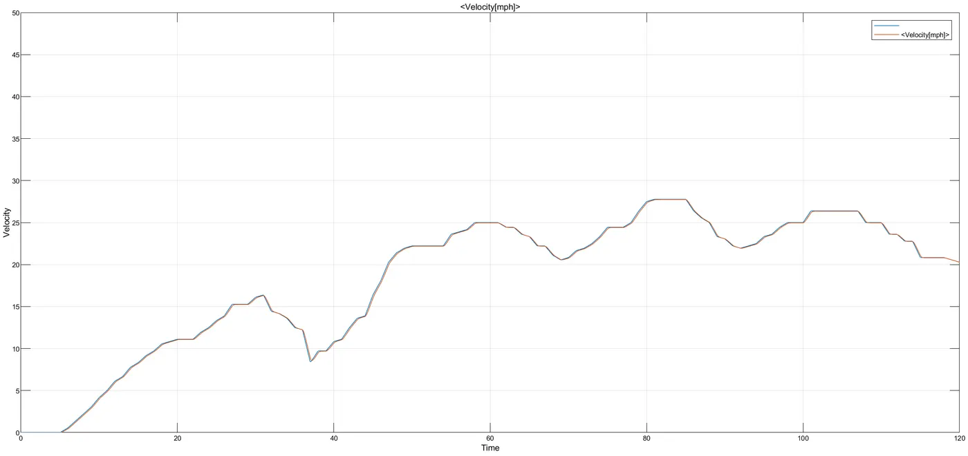
- Plot Time vs Velocity for 14Degrees Angle of Inclination.

4. Model the WOT (Wide Open Throttle) response of GM EV1 car:

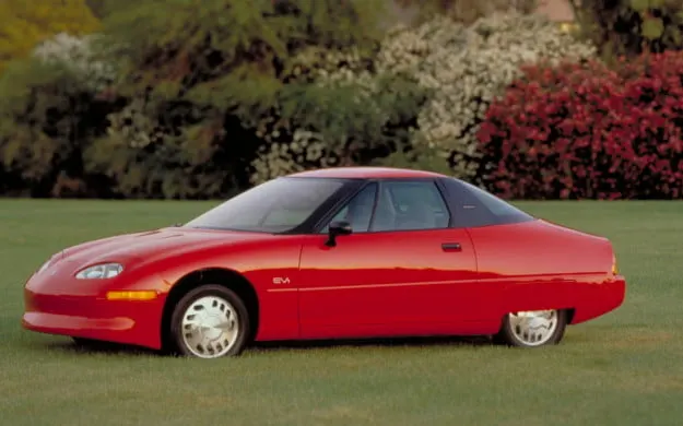
The GM EV1 was arguable the first modern electric car form the General Motors company it incorporated technologies that were quite noval for its time, and is indeed still unsurpassed as a design of a battery electeric car.

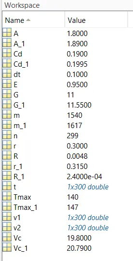
Vehicle parameters

• Drag Coefficient (Cd)
  Cd = 0.19

• Rolling Resistance (R)
  R=0.0048
  
  
• Vehicle Mass (m)
  m=1540 kg
  
  
• Gear Ratio (G)
  G= 11
  
  
• Radius of tire (r)
  r= 0.30
  
  
• Motor Torque (Tmax)
  Tmax=140 NM

• Motor Maximum speed = 12000 rpm

• Critical Velocity (Vc)
  Vc= 19.8 m/s
  
  
• Frontal Area (A)
  A=1.8 m^2

• Efficiency of single speed-drive
  E= 0.95
  
  

5% change in Vehicle parameters:

• • Drag Coefficient (Cd)
    Cd = 0.1995
  • Rolling Resistance (R)
    R=0.00024
    
    
  • Vehicle Mass (m)
    m=1617 kg
    
    
  • Gear Ratio (G)
    G= 11.55
    
    
  • Radius of tire (r)
    r= 0.315 m
    
    
  • Motor Torque (Tmax)
    Tmax=147 NM
  • Motor Maximum speed = 12600 rpm
  • Critical Velocity (Vc)
    Vc= 20.79 m/s
    
    
  • Frontal Area (A)
    A=1.89 m^2

Governing Equatons:

• Tractive Force:

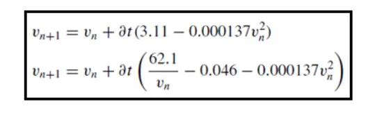
`Fte=μrr⋅mg+0.625ACdv2+ma+I*(G^2)/(mug*r^2)*a`

`G/r*T=``μrr⋅mg+0.625ACdv2+ma+I*(G^2)/(mug*r^2)*a``

MATLAB CODE:

% Wide Open Throttle (WOT) response for GM EV1 car
clear all
close all
clc

%Inputs
%Drag Coefficient (Cd)
Cd = 0.19;
%Rolling Resistance (R)
R=0.0048;
%Vehicle Mass (m) kg
m=1540; 
%Gear Ratio (G)
G= 11
%Radius of tire (r)
r= 0.30;
%Motor Torque (Tmax) NM
Tmax=140;
%Critical Velocity (Vc) m/s
Vc= 19.8;
%Frontal Area (A) m^2
A=1.8;
%Efficiency of single speed-drive 
E= 0.95;
%Time (t)
t= linspace(0,120,300);
%Initial Velocity (v1)
v1=0;
dt=0.1;
for n=1:299
    if v1(n)<19.8
        v1(n+1)= v1(n)+dt*(3.11-(0.00137*(v1(n)^2)));
    else if v1(n)>=19.8
            v1(n+1)=v1(n)+((62.1/(v1(n))-0.046-(0.000137*(v1(n)^2)))); 
        end
    end
end
%v1=v1*0.05;
%plotting
figure(1)
plot(t,v1);
title('WOT of GM EV1')
xlabel('Time (sec)')
ylabel('Velocity (m/s)')
grid on 



% Wide Open Throttle (WOT) response for GM EV1 car varied by 5%
%Inputs
%Drag Coefficient (Cd)
Cd = 0.1995;
%Rolling Resistance (R)
R=0.00024;
%Vehicle Mass (m) kg 
m=1617;
%Gear Ratio (G)
G= 11.55;
%Radius of tire (r)m
r= 0.315 
%Motor Torque (Tmax) NM
Tmax=147;
%Critical Velocity (Vc) m/s
Vc= 20.79;
%Frontal Area (A) m^2
A=1.89;
%Velocity
v2= (v1*0.05)+v1;

if v2(n)<19.8
    v2(n+1)=v2(n)+dt*(2.95-(0.000137*(v2(n)^2)));
else if v2(n)>=19.8
        v2(n+1)=v2(n)+dt*((59.14)/v2(n)-0.046-(0.000137*(v2(n)^2)));
    end
end
%Plotting
figure(2)
plot(t,v2,'color','r')
title('WOT of GM EV1 varied parameters by 5%')
xlabel('Time (sec)')
ylabel('Velocity (m/s)')
grid on 

figure(3)
plot(t,v1)
hold on
plot(t,v2,'color','r')
title('WOT of GM EV1')
legend('original parameters','5% varied Parameters')
xlabel('Time (sec)')
ylabel('Velocity (m/s)')
grid on

Procedure:

• Initially to Wide Open Throttle (WOT) response for GM EV1 car, the vehicle parameters are defined as per the provided data.
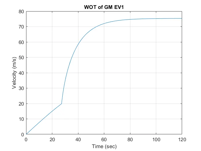
• Then, calculated the velocity with in the time span of 120 sec by providing the conditions of velocity as above.
• Then, Plotted the graph time vs velocity.
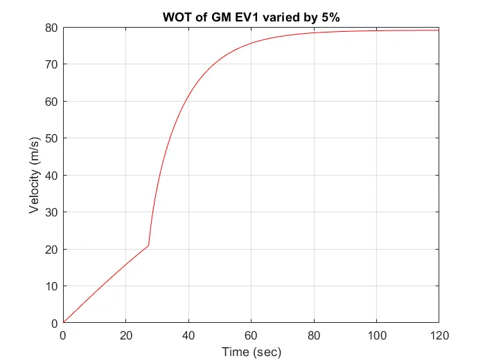
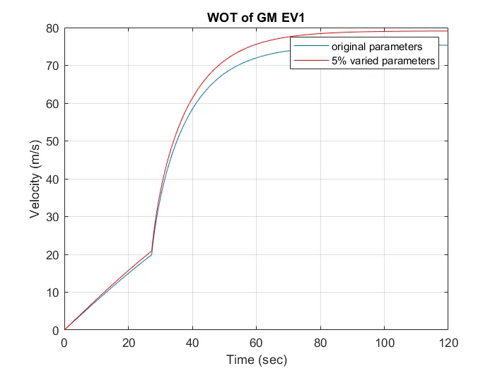
• Next, calculated the Wide Open Throttle (WOT) response for GM EV1 car, 5% change in velocity.
• And plotted the graphs for 5% change in velocity

Output:

• Workspace

• Plot for original parameters:

• Plot for 5% change in parameters

• Comparing 5% change in vehicle parameters with Original parameters

Conclusion:

Hence,

• Calculated the ratio of Hill-Climbing power required by fully loaded tata ultra truck to the half-loaded Truck.
• Calculated the minimum length of the flyover.
• Prepared a new drive cycle excel file and compared Driver Glider by changing the angle of inclination.
• Created a Model of WOT (Wide Open Throttle) response of GM EV1 car.

References:

• How to open DRIVER_GLIDER model in Simulink
• How to add drive cycle to the Driver glider model file in MATLAB
• How to model GM EV1 CAR for Wide open throttle calculation
• https://light-trucks.tatamotors.com/pdf/t16-ultra.pdf
• https://www.team-bhp.com/