Week 3 - Solving second order ODEs

Objective:

To write a program to solve the ODE that represents the equation of motion of a simple pendulum with damping and create animation.

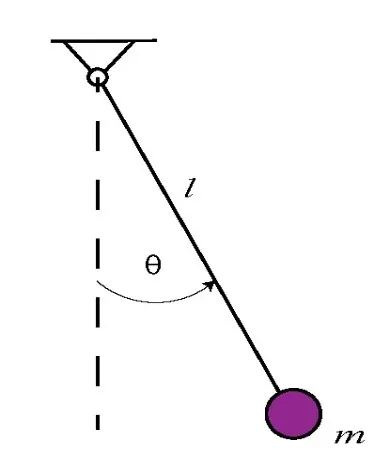
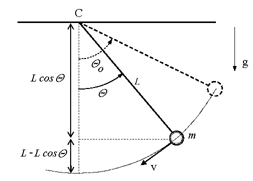
Schematic sketch of simple pendulum:

Simple pendulum ODE:

`(d^2theta)/dt^2+b/m*(d theta)/dt+g/l*sintheta=0`

where

`theta`= Angular displacemen`

`t`= Time (sec)`

`b=`damping coefficient`

`m=` mass (Kg)`

`g=` Accleration due to gravity (m/sec^2)`

`l=` Length of the string (m)`

Here time is independent variable and angular displacement is dependent variable. By solving second order ODE, will get different positions of pendulum w.r.t time.

After solving the given second order ODE, will convert into two first order ODE’s, which are:

`theta= theta1`

`(d theta1)/dt= theta2`

`(d^2 theta1)/dt^2=d/dt((d theta1)/dt)=(d theta2)/dt`

`(d theta2)/dt=-b/m*theta2-g/l*sin theta1`

Matlab code to simulate the pendulum motion:

%second order ODE_Simple pendulum
clear all
close all
clc

%inputs 
%Damping coefficient
b=0.05;
%Acceleration due to gravity (m/s^2)
g=9.81;
%Length of the string (m)
l=1;
%Mass of the bob (kg)
m=1;

%initial condition
%displacement & angular velocity
theta_0=[0;3];
%time points
t_span=linspace(0,20,500);

%soloving ODE
[t,results]=ode45(@(t,theta)ode_function(t,theta,b,g,l,m),t_span,theta_0);
%plotting 
figure(1)
plot(t,results(:,1),'linewidth',3)
hold on
plot(t,results(:,2),'linewidth',3)
xlabel('time-sec')
ylabel('angular velocity & displacement')
legend('change in dispnacement','change in angular velocity')
hold off
grid on
figure(2)
theta2=results(:,1);
ct=1;
for i=1:length(theta2);
    theta3=theta2(i);
    x0=0;y0=0;
    x1=l*sin(theta3);
    y1=-l*cos(theta3);
 
    plot([x0 x1],[y0 y1],'linewidth',3);
    axis([-1 1 -1.5 0.5])
    hold on
    plot(x1,y1,'marker','o','markersize',20,'markerfacecolor','r')
    hold off
    grid on 
    pause(0.1)
    M(ct)=getframe(gcf);
    ct=ct+1;
end
%creating movie
movie(M)
videofile=VideoWriter('pendulum.avi','Uncompressed AVI');
open(videofile)
writeVideo(videofile,M)
close(videofile)

%ODE function
function[dtheta_dt]=ode_function(t,theta,b,g,l,m)
theta1= theta(1);
theta2= theta(2);
dtheta_dt=theta2;
dtheta2_dt=-(b/m)*theta2-(g/l)*sin(theta1);
dtheta_dt=[dtheta1_dt;dtheta2_dt];
end

Explanation:

• Initially, I have defined the finction code by using ODE function.

Procedure:

• Initially Define the inputs i.e., damping coefficient(b), acceleration due to gravity(g), length of the string(l), mass of the ball(m).
• Define initial condition for angular displacement, angular velocity and time span.
• Define the function in terms of “t &theta” separately by using two first order equations solved.
• To solve the ODE select the ‘ode45’ matlab solver and call the function defined separately.
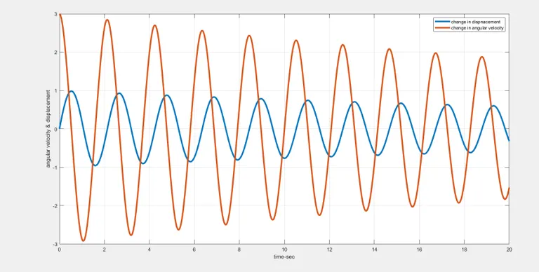
• Figure 1: Plot the graph ‘time Vs angular displacement& angular velocity’.
• Figure 2: ‘for loop’ is used to create motion of pendulum. In the for loop ‘i’ is assigned for angular displacement in terms of theta2. And theta2 (i) value is assigned to theta3, then the initial values of ball are assigned. And the position of the string traced by the “l*sin theta3 and l*cos theta3”. And the plotting string on graph. Next will specify the required axis limits and hold on. Then by using marker command the sphere is created. Next will specify the required pause time at each position. Next by using ‘getframe’ command and ‘ct’-increment will create frame and increase the position. Next will end the loop.
• Finally create the movie videofile and store in the “avi” format.
• Publish the animation of simple pendulum.

Commands used in the program:

• ‘linspace’ command to define time span of pendulum.
• ‘Plot’ command to plot the graphs.
• ‘marker’ command to create the sphere(ball).
• ‘movie’ command to create the movie.
• ‘VideoWriter’ command to create AVI file.

ode45:

‘ode45’ is a function in matlab that solves the ordinary differential equations using a numerical method. The numerical method used here is second order differential equation.

Generally to solve an ODE we need to integrate and solve for the variable. Instead we can use the numerical solver, by discretising the equation into linear equation and then solve the equation to approximate the solution.

Any ODE to be integrated by ode45 must be provided as a set of first order ODEs.

The function ode45 takes 3 inputs. Which are function to be integrated, the time span and the initial conditions.

• The time span would be the integrated limits. This can be provided as a vectors of 2 values, the initial and final time or the spacing using the ‘linspace’ command. The solver will choose the step size that is most suitable for the solution to obtain the solution in the most optimal time as possible.
• The initial conditions would be the value of the function at t=0sec.
• The function can be provided in the anonymous function,

Syntax of ode45: [t,results]=ode45(@(t,y) ode_func(t,y,arguments),tspan,y0)

Output:

• Plot: Time Vs Angular displacements & angular velocity.

• Animation of simple pendulum:

https://www.youtube.com/watch?v=IuzH1H8RX80

https://drive.google.com/file/d/1mTfnZ7A55elKLPjTGOWm9N8wAGEPnA58/view?usp=sharing

Conclusion:

Hence the Animation of simple pendulum is done and published.