Week 4 - Genetic Algorithm
Objective:
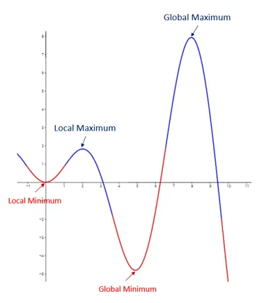
To write a code in MATLAB to optimise the stalagmite function and find the global maxima of the function. And Understand the process of GA.
Theory:
Introduction to Optimization:
The field of optimization has evolved significantly over the past few decades. Several new theoretical, algorithmic, and computational methods for optimization have been proposed to solve complex problems in diverse fields such as finance, engineering and molecular biology.
Optimization methods can be divided into two primary categories;
Deterministic and Heuristic approaches. Both methods are essential for quantitative finance applications.
Deterministic optimization is a highly mathematical and gradient-based form of optimization that is most suitable for well-defined problems that contain a smooth and continuous search space. Some examples of deterministic optimization would be conjugate gradient, simplex, gradient descent, quadratic- programming, non-linear solvers, and quasi-Newton or Newton methods. These methods are greedy and highly efficient, and if used for the appropriate application they are guaranteed to find the global optimum. Deterministic methods are analogous to Formula One race cars
Heuristic approaches in contrast are either algorithmic or stochastic and can be used for highly complex problems without the need for expert knowledge. Traditional examples of heuristic methods would be Monte Carlo (MC), particle-swarm optimization (PSO), genetic algorithms (GA), simulated annealing (SA), and differential evolution. The class of algorithmic heuristic approaches are typically domain specific (or even specific purpose) and less generalizable than stochastic methods. Most scientists and engineers find heuristic methods to be more flexible and efficient than deterministic approaches for complex real-world problems, but finding the global optimum cannot be guaranteed. However, in a typical large-scale application a true exhaustive search is either not possible or practical from a computation standpoint.
Genetic Algorithm (GA):
A Genetic Algorithm (GA) is a heuristic search technique used in computing to find true or approximate solutions to optimization and search problems. This algorithm reflects the process of natural selection where the fittest individuals are selected for reproduction in order to produce offspring of the next generation.
The process of natural selection starts with the selection of fittest individuals from a population. They produce offspring which inherit the characteristics of the parents and will be added to the next generation. If parents have better fitness, their offspring will be better than parents and have a better chance at surviving. This process keeps on iterating and at the end, a generation with the fittest individuals will be found.
Genetic algorithm developed by Goldberg was inspired by Darwin's theory of evolution which states that the survival of an organism is affected by rule "the strongest species that survives". Darwin also stated that the survival of an organism can be maintained through the process of reproduction, crossover and mutation. Darwin's concept of evolution is then adapted to computational algorithm to find solution to a problem called objective function in natural fashion. A solution generated by genetic algorithm is called a chromosome, while collection of chromosomes is referred as a population.
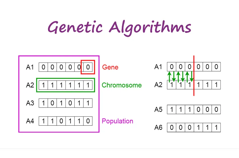
Five phases are considered in a genetic algorithm.
- Initial population
- Fitness function
- Selection
- Crossover
- Mutation
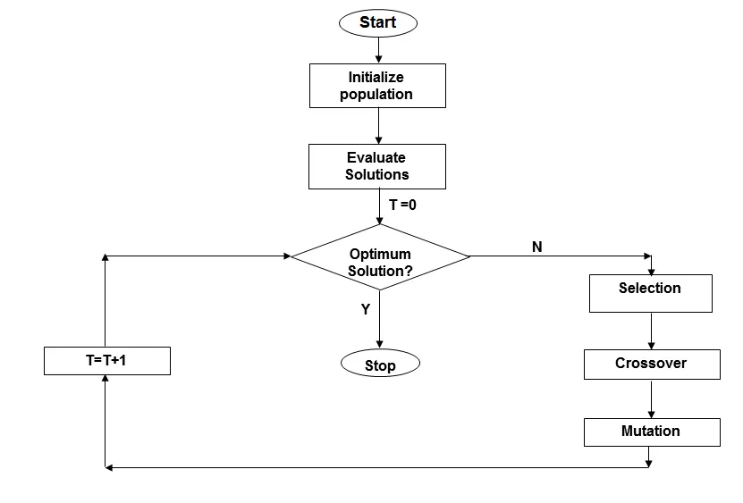
Genetic Algorithm Syntax:
[x,fval,exitflag,output,pop,scores]=ga(fun,nvars,A,b,Aeq,beq,lb,ub,nonlcon,intcon,options)
Where,
x= optimum solutions
fval= function evaluation
exitflag= reason GA to stopped
output= information about optimization process
pop= final population
scores= final scores
fun= fitness function
nvars= no. of variables
A,b= linear inequality constrains
Aeq,beq= linear equality constrains
lb= lower bound(limit)
ub= upper bound(limit)
nonlcon= use for nonlinear constrains
Intcon= to get solution in integeras
options= to get population size minimum with non-default options
Stalagmite & Stalactites:
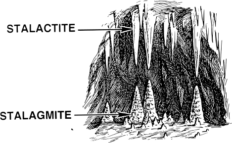
- Stalactites hang from the ceiling of a cave while stalagmites grow from the cave floor. A stalactite is an icicle-shaped formation that hangs from the ceiling of a cave and is produced by precipitation of minerals from water dripping through the cave ceiling. Most stalactites have pointed tips. A stalagmite is an upward-growing mound of mineral deposits that have precipitated from water dripping onto the floor of a cave. Most stalagmites have rounded or flattened tips.
Stalagmite Fitness function:
`f(x,y)=f1x*f2x*f1y*f2y`
`f1x=[sin(5.1pix+0.5)]^6`
`f1y=[sin(5.1piy+0.5)]^6`
`f2x=exp[-4ln(2)(x-0.0667)^2/0.64]`
`f2y=exp[-4ln(2)(y-0.0667)^2/0.64]`
Body of content:
Matlab code:
Function code:
%stalagmite function for GA
function [f]= stalagmite(input_vector)
x1=input_vector(1);
y1=input_vector(2);
f_1x=(sin((5.1*pi*x1)+0.5))^6;
f_1y=(sin((5.1*pi*y1)+0.5))^6;
f_2x= exp((-4*(log(2))*(x1-0.0667)^2)/0.64);
f_2y= exp((-4*(log(2))*(y1-0.0667)^2)/0.64);
f=-(f_1x*f_1y*f_2x*f_2y); %-ve sign indicates for global maxima
end
Study_1:
clear all
close all
clc

%Defining our search space
x=linspace(0,1,100);
y=linspace(0,1,100);
n=50; %no.of itarations

%study1: statical behaviour of GA
%Creating 2D mesh
[xx,yy]=meshgrid(x,y);
%Evaluating the stalagmite function
for i=1:length(xx)
    for j=1:length(yy)
        input_vector(1)= xx(i,j);
        input_vector(2)= yy(i,j);
        f(i,j)= stalagmite(input_vector);
    end
end


tic
for k=1:n
    [inputs,fopt(k)]=ga(@stalagmite,2);
    xopt(k)=inputs(1);
    yopt(k)=inputs(2);
end
study_time1= toc
%plotting
figure(1)
subplot(2,1,1)
surf(x,y,-f)
shading interp
xlabel('x')
ylabel('y')
title('case1')
hold on
plot3(xopt,yopt,-fopt,'marker','o','markersize',5,'markerfacecolor','r')
title('unbounded inputs')
subplot(2,1,2)
plot(fopt)
xlabel('itrations')
ylabel('function maxima')
Explanation:
The main objective is to optimize the stalagmite function.
Before writing the main code, I have defined stalagmite function by the fitness function governing equations.
- In the main code Initially I have defined the search space of x, y by using the linspace() command. And also defined no. of iterations.
- Then I have created 2D mesh using meshgrid() command.
- Next, I have evaluated the stalagmite function using 2 ‘for’ loops for x & y variables.
Procedure for study_1:
- In the first study I have coded for statistical behaviour of the function without specifying any boundaries.
- I have used tic and toc command to check run time (how much time the matlab is taking to run the code). And initiated the no. of iterations to perform.
- And used ‘for’ loop to initiate the inputs by using genetic algorithm.
- Next, I have plotted for the unbounded inputs. In this plot I have two created subplots by using subplot() command; first half of plot is for stalagmites-to find the global maxima and the second one half is to show the iterations performed against function maxima.
- By using Surf() command, I have created a three-dimensional surfaceplot, which is a three-dimensional surface that has solid edge colors and solid face colors.
- Shading interp() command is used for smooth display of stalagmites, without any interruption (to avoid grid lines on the stalagmites).
- Then after the coding is done, I have run the program.
output:
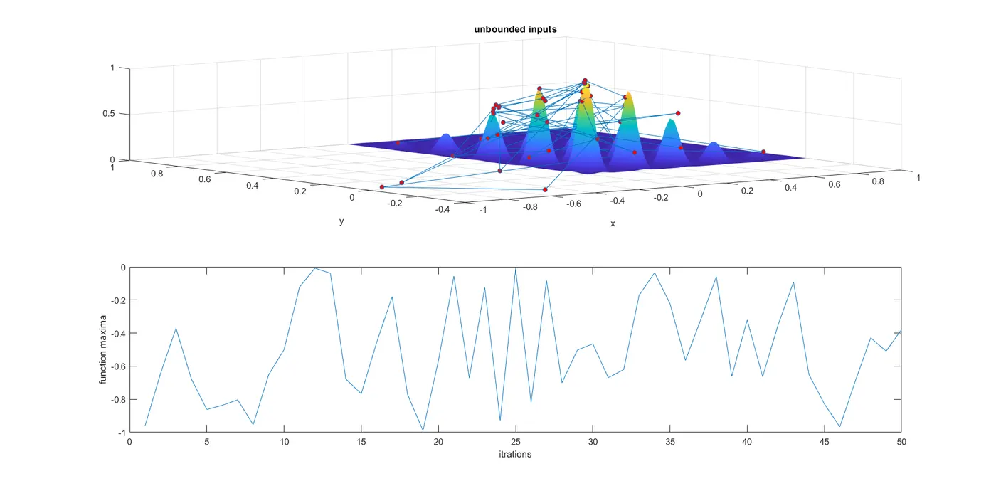
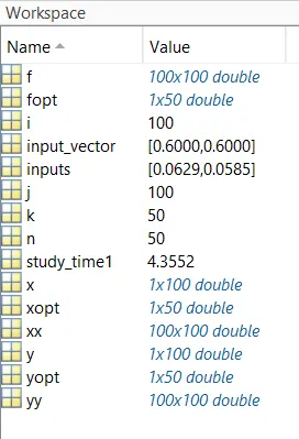
- In the first stage we are unable to find the global maxima. To optimise this, I have run the second study by providing the boundary limits to it.
Study_2:
clear all
close all
clc

%Defining our search space
x=linspace(0,1,100);
y=linspace(0,1,100);
n=50; %no.of itarations
%Creating 2D mesh
[xx,yy]=meshgrid(x,y);
%Evaluating the stalagmite function
for i=1:length(xx)
    for j=1:length(yy)
        input_vector(1)= xx(i,j);
        input_vector(2)= yy(i,j);
        f(i,j)= stalagmite(input_vector);
    end
end

%study2: statical behaviour of GA with upper and lower bounds
tic
for k=1:n
    [inputs,fopt(k)]=ga(@stalagmite,2,[],[],[],[],[0;0],[1;1]);
    xopt(k)=inputs(1);
    yopt(k)=inputs(2);
end
study_time2= toc
%plotting
figure(2)
subplot(2,1,1)
surf(x,y,-f)
hold on
shading interp
xlabel('x')
ylabel('y')
title('study2')
plot3(xopt,yopt,-fopt,'marker','o','markersize',5,'markerfacecolor','r')
title('bounded inputs')
subplot(2,1,2)
plot(fopt)
xlabel('itrations')
ylabel('function maxima')
Procedure for study_2:
- To get the optimized results I have created second study with providing the upper and lower boundaries in GA.
- Similarly as the study_1, I have used tic and toc command to check run time (how much time the matlab is taking to run the code). And initiated the no. of iterations to perform.
- And used ‘for’ loop to initiate the inputs by using genetic algorithm.
- Next, I have plotted for the unbounded inputs. In this plot I have two created subplots by using subplot() command; first half of plot is for stalagmites-to find the global maxima and the second one half is to show the iterations performed against function maxima.
- By using Surf() command, I have created a three-dimensional surfaceplot, which is a three-dimensional surface that has solid edge colors and solid face colors.
- Shading interp() command is used for smooth display of stalagmites, without any interruption (to avoid grid lines on the stalagmites).
- Then after the coding is done, I have run the program.
Output:
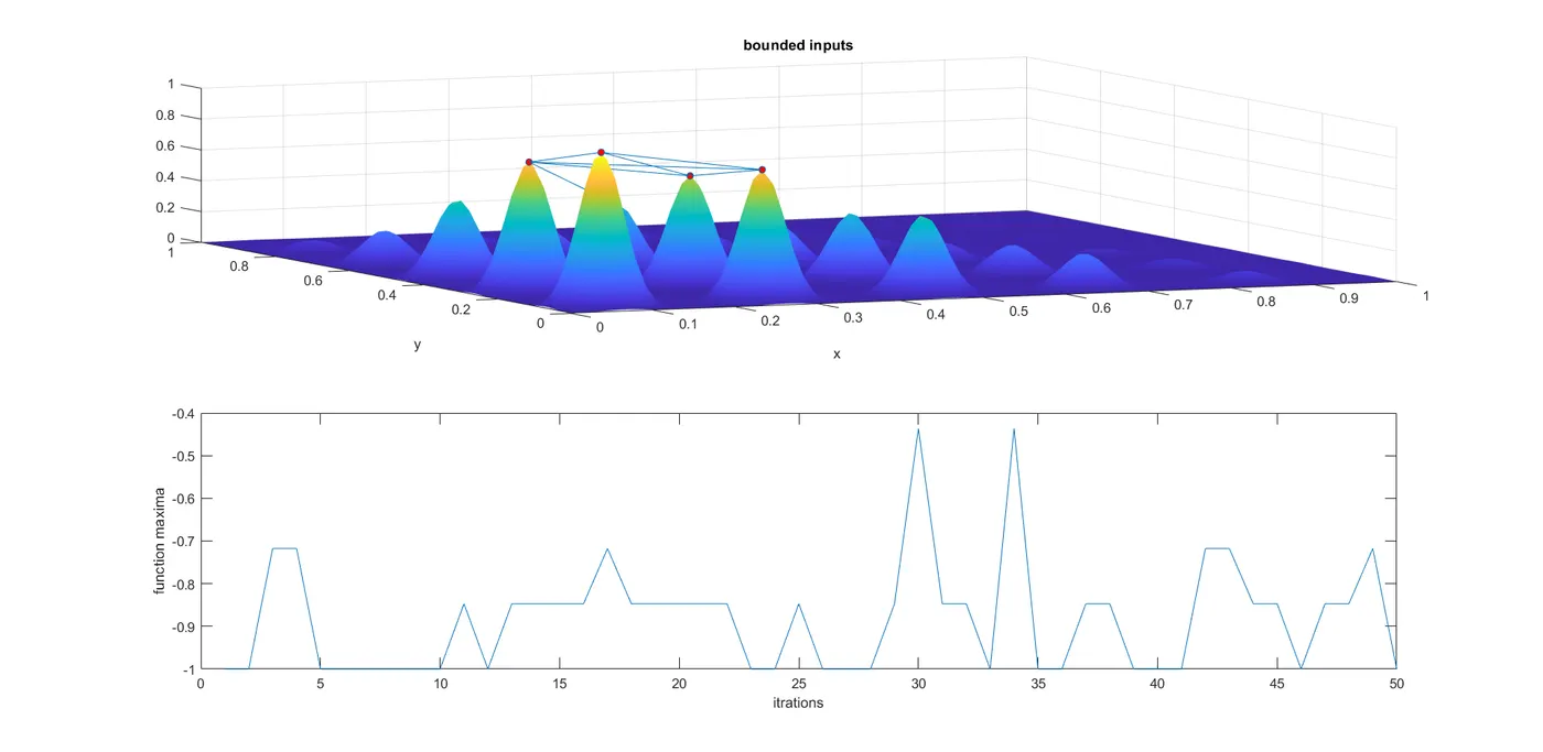
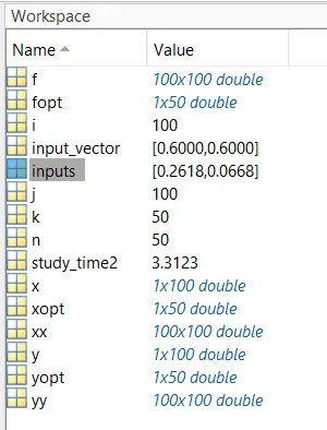
- The above plot is generated for study_2.
- Even after the specifying the boundary limits, the value is not optimum.
Study_3:
%Optimising the stalagmite function by GA
clear all
close all
clc

%Defining our search space
x=linspace(0,1,100);
y=linspace(0,1,100);
n=50; %no.of itarations
%Creating 2D mesh
[xx,yy]=meshgrid(x,y);
%Evaluating the stalagmite function
for i=1:length(xx)
    for j=1:length(yy)
        input_vector(1)= xx(i,j);
        input_vector(2)= yy(i,j);
        f(i,j)= stalagmite(input_vector);
    end
end
%study3: statical behaviour of GA by incresing the no of itrations
 options=optimoptions('ga');
 options=optimoptions(options,'populationsize',500);
tic
for k=1:n
    [inputs,fopt(k)]=ga(@stalagmite,2,[],[],[],[],[0;0],[1,1],[],options);
    xopt(k)=inputs(1);
    yopt(k)=inputs(2);
end
study_time3= toc
%plotting
figure(3)
subplot(2,1,1)
surf(xx,yy,-f)
hold on
shading interp
xlabel('x')
ylabel('y')
title('case3')
plot3(xopt,yopt,-fopt,'marker','o','markersize',5,'markerfacecolor','r')
title('bounded inputs with modified populationsize')
subplot(2,1,2)
plot(fopt)
xlabel('itrations')
ylabel('function maxima')
display(inputs) %Displaying the values of x & y for maximum value of function
Procedure for study_3:
- In the study_3, I have increased the iterations and population size by using optimoptions() command.
- And the rest of the procedure is similar to study_1 and study_2.
- In the end I have used display() command to display the inputs/optimum value.
- And then run the program.
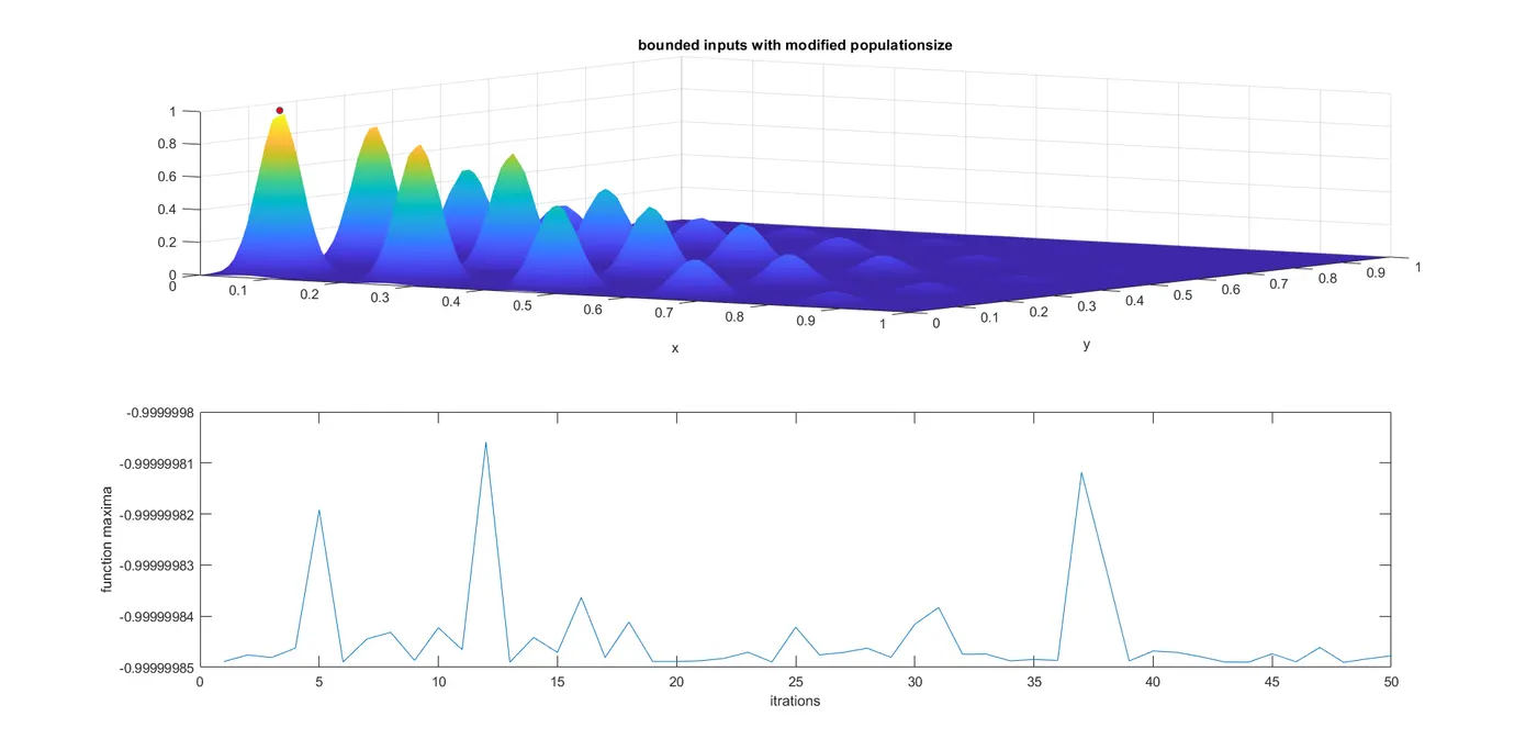
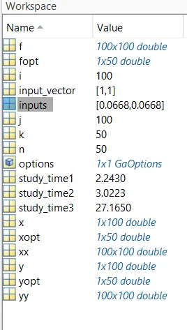
Output:
Results:
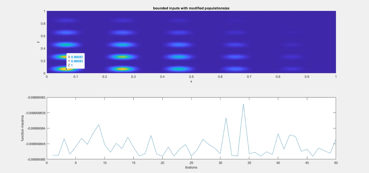
- The function is optimized.
- The global maxima value is [0.0668, 00.0668]
Conclusion:
Hence the stalagmite function is optimized and find the global maxima.
Reference:
- https://www.iitg.ac.in/rkbc/CE602/CE602/Genetic%20Algorithms.pdf
- https://www.researchgate.net/profile/Colin_Reeves
- https://www.researchgate.net/publication/226462334_Genetic_Algorithms
- https://oceanexplorer.noaa.gov/welcome.html
- https://www.onlinemathlearning.com/
- https://towardsdatascience.com/@vijinimallawaarachchi?source=post_page-----e396e98d8bf3----------------------