Curve Fitting

Objective:

1. To write a code to fit a linear and cubical polynomial for the Specific Heat(cp) data.
2. To write a code to show splitwise method.
3. To explain the Parameters used to measure the fitness characteristics for the both the curves.

Theory:

Curve fitting:

Curve fitting is a process of constructing a curve, or mathematical function, which possess the closest proximity to the real set of data. By curve fitting, we can mathematically construct the functional relationship between the observed dataset and parameter values.

We identify the nature of a relationship between two variables by examining if the points on the scatter plot conform to a linear, exponential, quadratic, cubic or some other function. The strength of a relationship can be described as strong if the data points conform closely to a function or weak if they are further away.

The goodness of fit of a set of data determines how proximately it fits a set of observations.

Parameters that used to measure the fitness characterises of both the curves

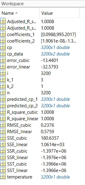
1. The sum of squares due to error (SSE): Summation of square of all errors(difference between original value and predicted value)

`SSE=``sum i=1 to n (y(i)-f(x(i))^2)`

where, `y(i)=`original data

`f(x(i))=`predicted data

2. R_square `(R^2)=(SSR)/(SST)`

where,

sum of squares of the regression (SSR)=`sumi=1 to n (f(x(i))-Mean)^2`

SST= SSR+SSE

3. Adjusted `(R^2)adj=1-[((1-R^2).(n-1))/(n-k-1) ]`

where, k= no.of data points

n= no.of independent variables

4. Root Mean Square Error(RMSE):This statistic is also known as the fit standard error and the standard error of regression. It is an estimation of standard deviation of a random component in the data and is defined as,

RMSE= `sqrt ((SSE)/n)`

How to make a curve fit perfectly?

• Perfect fit means to fit the curve perfectly to the set of original data without any errors. To make a curve fit perfect, we need to consider error estimations.
• We can also change the order of polynomial to get the perfect fit. By increasing the order of the polynomial, the curve fits perfectly to the original data.

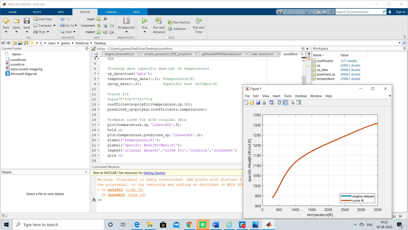
• In the above slide I have increased to 10 order polynomial and the curve is fitted perfectly.

How to get a best fit?

• To get the best fit we can consider the R_square and RMSE if the R_square value is >0.955, then it is called best fit.
• R_square = 0 is consider as a worst fit.
• R_square = 1 is the best possible fit.

Note: perfect fit can always a best fit, but best fit can’t be the perfect fit.

• What could be done to improve the cubic fit?
• By splitwise method we can improve the cubic fit. In the splitwise method will split the data into more than two sets and evaluate.

Matlab polynomial functions:

• Polyvalv() = evaluate polynomial
• Polyint() = integrate polynomial
• Polyfit() = least squares polynomial curve fit
• Polyder = derivate of polynomial
• Roots = return roots of a polynomial
• Conv = multiply of two polynomial
• Deconv = divide two polynomials

Program:

Matlab code of linear and cubical polynomial:

%curve fit for cp data_Linear and cube polynomial
clear all
close all
clc

%loading data (specific Heat(cp) Vs Temperature)
cp_data=load('data'); 
temperature=cp_data(:,1); %temperature[K]
cp=cp_data(:,2);          %specific heat [KJ/Kmol-K]

figure(1)  %linear polynomial curve fit
%cp=a*T+b   %y=m*x+c
coefficients_1=polyfit(temperature,cp,1); %coffficients of polynomial are generated using polyfit() command
predicted_cp_1=polyval(coefficients_1,temperature); %predected values of cp_1 are generated using polyval() command

%compare curve fit with original data
plot(temperature,cp,'linewidth',3); %original data set
hold on
plot(temperature,predicted_cp_1,'linewidth',3);
xlabel('temperature[K]');
ylabel('specific Heat[KJ/Kmol-K]');
legend('original dataset','curve fit','location','southeast')
title('linear polynomial curve fit')
grid on

figure(2)  %cubie polynomial curve fit
%cp=a*T^3+b*T^2+c*T+d
coefficients_2=polyfit(temperature,cp,3); %coffficients of polynomial are generated using polyfit() command
predicted_cp_2=polyval(coefficients_2,temperature); %predected values of cp_2 are generated using polyval() command

%compare curve fit with original data
plot(temperature,cp,'linewidth',3); %original data set
hold on
plot(temperature,predicted_cp_2,'linewidth',3); %plotting
xlabel('temperature[K]');
ylabel('specific Heat[KJ/Kmol-K]');
legend('original dataset','curve fit','location','southeast')
title('cube polynomial curve fit');
grid on


%choosing best fit
%fitness characteristics for linear curve fit
n=3200; %no.of data points
k_1=3; %no.of independent variables
for i = 1:length(cp); 
    error_linear = cp(i)-predicted_cp_1(i);
    SSE_linear = sum(error_linear).^2;   %sum of squares due to error
    SSR_linear = sum(predicted_cp_1(i)-mean(cp).^2);  %sum of squares of the regression
end
%goodness of fit
SST_linear = (SSR_linear+SSE_linear);
R_square_linear = (SSR_linear/SST_linear);
Adjusted_R_square_linear = 1-((1-R_square_linear)*(n-1)/(n-k_1-1));
RMSE_linear = sqrt(SSE_linear/n);

%fitness characteristics for cubic curve fit
k_2=1; %no.of independent variables
for i = 1:length(cp); 
    error_cubic = cp(i)-predicted_cp_2(i);
    SSE_cubic = sum(error_cubic).^2;   %sum of squares due to error
    SSR_cubic = sum(predicted_cp_2(i)-mean(cp).^2);  %sum of squares of the regression
end
%goodness of fit
SST_cubic = (SSR_cubic+SSE_linear);
R_square_cubic = (SSR_cubic/SST_cubic);
Adjusted_R_square_cubic = 1-((1-R_square_cubic)*(n-1)/(n-k_2-1));
RMSE_cubic = sqrt(SSE_cubic/n);

Procedure:

• Initially I have loaded the cp data by using ‘load()’ command.
• Next defined the temperature and cp values
• Figure 1: Linear polynomial curve fit
• coefficients of polynomials are generated by using polyfit() command. Next I have predicted the value of cp_1 using polyvalv() command.
• Next I have plotted original dataset and predicted dataset by plot() command & compared the original dataset and predicted data for the linear polynomial curve fit.
• Figure 2: cubic polynomial curve fit

Similarly as the linear polynomial curve fit I have compared cubic curve fit with the original data using polt() command.

Output:

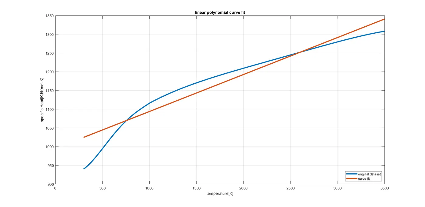
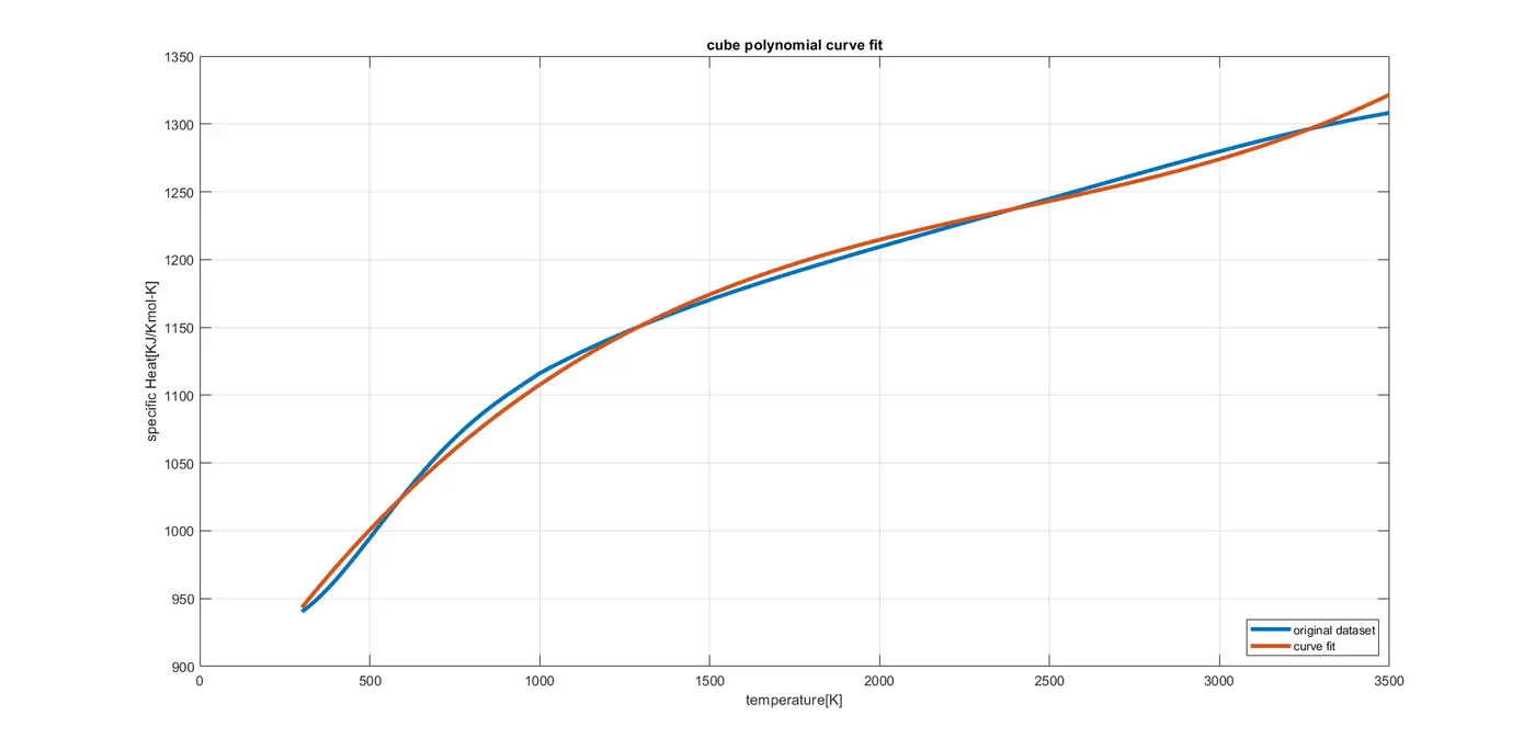
• The linear and cubic polynomial curves was plotted in fig1 & fig2 separately.
• Output plots was shown in the results.

1. Linear polynomial curve fit plot

2. Cubic polynomial curve fit plot

Matlab code for splitwise method:

%splitwise method curve fit
clear all
close all
clc

%loading data (specific Heat(cp) Vs Temperature)
cp_data=load('data');
temperature=cp_data(:,1); %temperature[K]
cp=cp_data(:,2);          %specific heat [KJ/Kmol-K]

%Splitting the data into 4 equal sets
temperature_1 = cp_data(1:800,1); 
cp_1 = cp_data(1:800,2);  
coefficients_1 = polyfit(temperature_1,cp_1,3); %coffficients of polynomial are generated using polyfit() command
predicted_cp_1 = polyval(coefficients_1,temperature_1);

temperature_2 = cp_data(801:1600,1); 
cp_2 = cp_data(801:1600,2);  
coefficients_2 = polyfit(temperature_2,cp_2,3); %coffficients of polynomial are generated using polyfit() command
predicted_cp_2= polyval(coefficients_2,temperature_2);%predected values of cp are generated using polyval() command

temperature_3 = cp_data(1601:2400,1); 
cp_3 = cp_data(1601:2400,2);  
coefficients_3 = polyfit(temperature_3,cp_3,3); %coffficients of polynomial are generated using polyfit() command
predicted_cp_3 = polyval(coefficients_3,temperature_3); %predected values of cp are generated using polyval() command

temperature_4 = cp_data(2401:3200,1); 
cp_4 = cp_data(2401:3200,2);  
coefficients_4 = polyfit(temperature_4,cp_4,3); %coffficients of polynomial are generated using polyfit() command
predicted_cp_4 = polyval(coefficients_4,temperature_4); %predected values of cp are generated using polyval() command

%plotting
plot(temperature,cp,'linewidth',3); %original data set
hold on

%Splitwise method data set
predicted_cp = [predicted_cp_1;predicted_cp_2;predicted_cp_3;predicted_cp_4]; %combined predicted_cp
plot(temperature,predicted_cp,'linewidth',3); %plotting 
xlabel('temperature[K]');
ylabel('specific Heat[KJ/Kmol-K]');
legend('original dataset','curve fit','location','southeast')
title('Splitwise method curve fit');
grid on


%choosing best fit
n=3200; %no.of data points
k=3; %no.of independent variables
for i = 1:length(cp); 
    error_splitwise = cp(i)-predicted_cp(i);
    SSE_splitwise = sum(error_splitwise).^2;   %sum of squares due to error
    SSR_splitwise = sum(predicted_cp(i)-mean(cp).^2);  %sum of squares of the regression
end 

%goodness of fit
SST_splitwise = (SSR_splitwise+SSE_splitwise);
R_square_splitwise = (SSR_splitwise/SST_splitwise)
Adjusted_R_square_splitwise = 1-((1-R_square_splitwise)*(n-1)/(n-k-1))
RMSE_splitwise = sqrt(SSE_splitwise/n)

Procedure:

• Initially I have loaded the cp data using load() command.
• Next defined temperature and cp values.
• To improve the cubic fit, I have spited the whole data into 4 equal parts.
• In each part I have defined coefficients of polynomial and predicted cp w.r.t temperature.
• Next I have plotted original dataset by plot() command
• Next combined 4 parts of cp and temperature dataset into single set of predicted data and plotted the predicted data.
• Next, I have compared predicted data and original data.
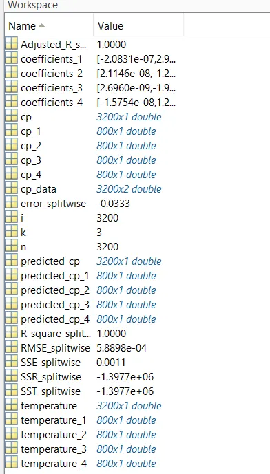
• Next, calculated the R_square, Adjusted R_square and RMSE to check the goodness of curve fit.

Output:

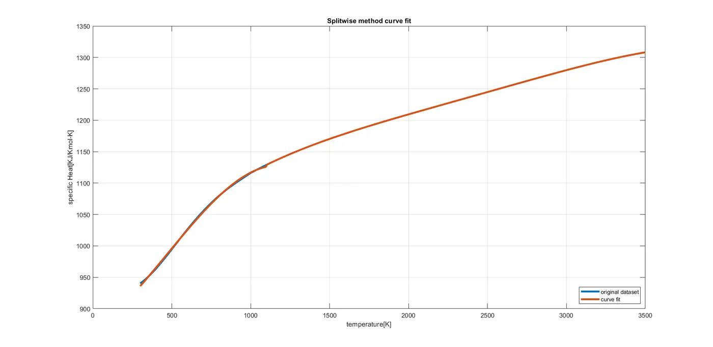
• The cubic curve was fitted perfectly with the original data.
• And the R_square value is equal to 1. Which indicates is as a good fit.

Conclusion:

Created linear polynomial curve fit & cubic polynomial curve fit and to improve the cubic polynomial fit I used splitwise method.

Hence the curve fitted perfectly.

Reference:

• https://projects.skill-lync.com/projects/Curve-Fitting-and-criterion-to-choose-best-fit-41860
• https://www.youtube.com/watch?v=LP0YrsMGMAM&list=LL4zf37mQ8zpmII19p3_uvvQ&index=5&t=0s