Conjugate Heat Transfer Analysis on a graphics card.

Aim :

To perform CHT analysis on a graphics card using ANSYS-FLUENT

Introduction :

A Graphics Card is a piece of computer hardware that produces the image you see on a monitor. They can be integrated with the computer processor. or can be added externally as a dedicated graphics card in a PC. As it is an electronic device, it must generate heat and hence we have to analyze its heat flow otherwise it may hurt the other parts of computers. In this project was simulation was performed on two meshes. First with automatically generated mesh and others with the refined mesh while maintaining y+.

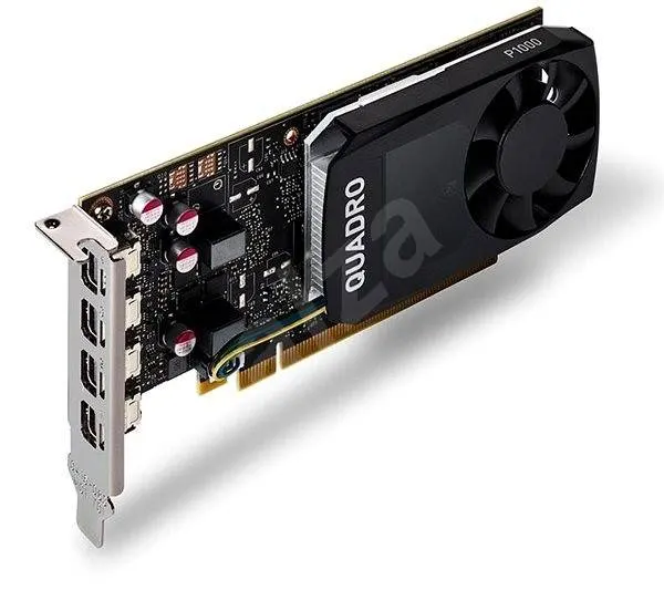
Picture of a real graphics card :

Theory :

The contemporary conjugate convective heat transfer model was developed after computers came into wide use in order to substitute the empirical relation of proportionality of heat flux to temperature difference with heat transfer coefficient which was the only tool in theoretical heat convection since the times of Newton. This model, based on a strictly mathematically stated problem, describes the heat transfer between a body and a fluid flowing over or inside it as a result of the interaction of two objects. The physical processes and solutions of the governing equations are considered separately for each object in two subdomains. Matching conditions for these solutions at the interface provide the distributions of temperature and heat flux along the body–flow interface, eliminating the need for a heat transfer coefficient.

One simple way to realize conjugation is to apply the iterations. The idea of this approach is that each solution for the body or for the fluid produces a boundary condition for other components of the system. The process starts by assuming that one of the conjugate conditions exists on the interface. Then, one solves the problem for the body or for fluid applying the guessing boundary condition and uses the result as a boundary condition for solving a set of equations for another component, and so on. If this process converges, the desired accuracy may be achieved. However, the rate of convergence highly depends on the first guessing condition, and there is no way to find a proper one, except through trial and error.

Solving & Modelling approach :

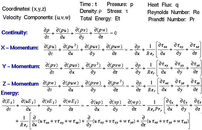
Governing Equations :

Materials :

Components	Material	Density `((kg)/(m^3))`	`C_p` `(J/(Kg-K))`	K `(W/(m-K))`
Processor	Silicon	2330	705	148
Fins	Aluminum	2719	871	202.4
PCB	Thermoplastic -ABS	1050	1390	0.25
Fluid	Air	1.225	1006.43	0.0242

The simulation is performed for two meshes and three different velocities.

These velocities are 1,3,5 `m*s^-1`

Mach number is very less for all of them, So it's an incompressible fluid flow

Pre-processing and solver setting :

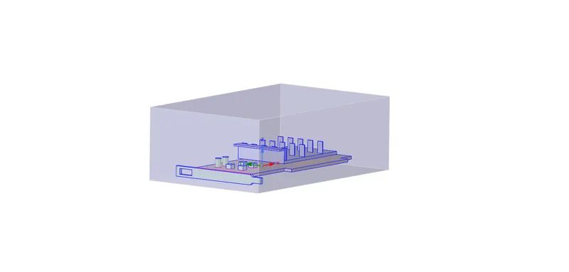
Geometry

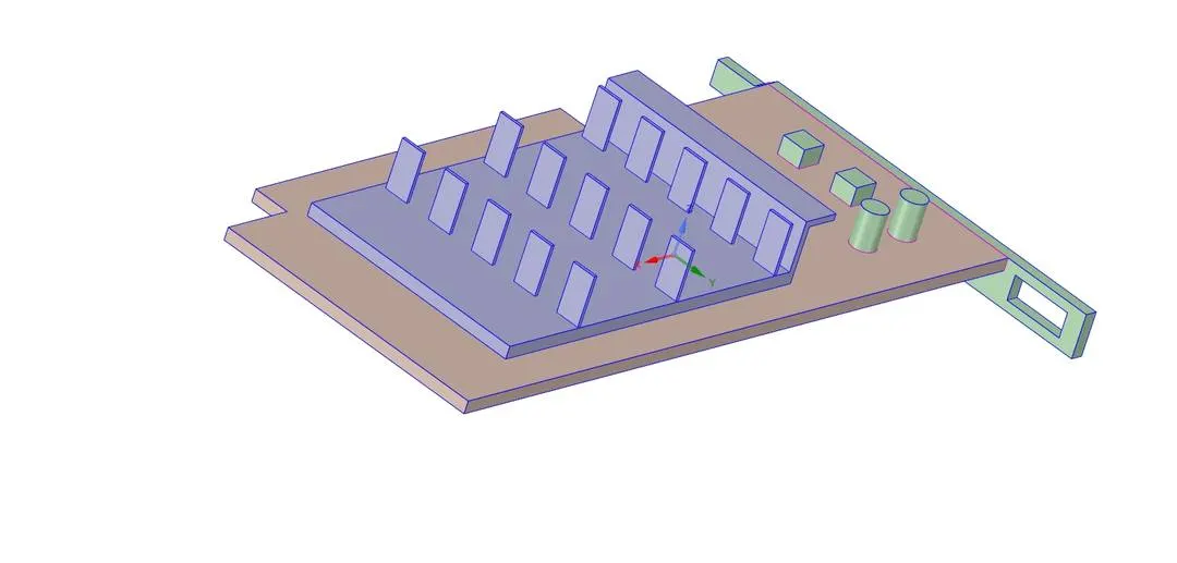
Graphics Card

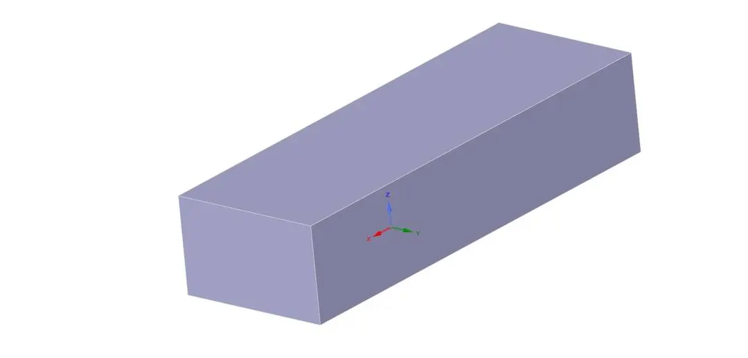
Outer Enclosure

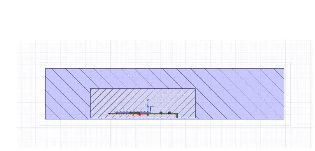
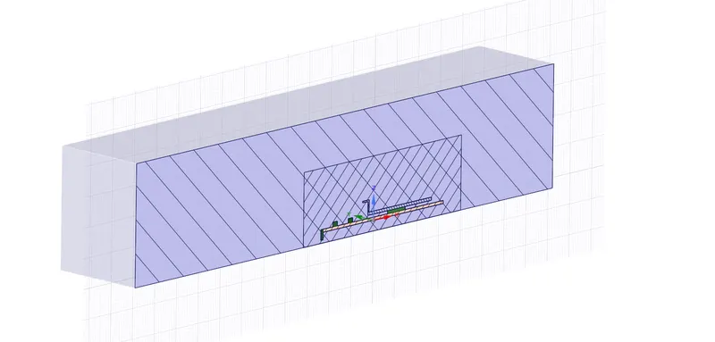
Inner Enclosure(For Mesh2)

Interference(For Mesh2)

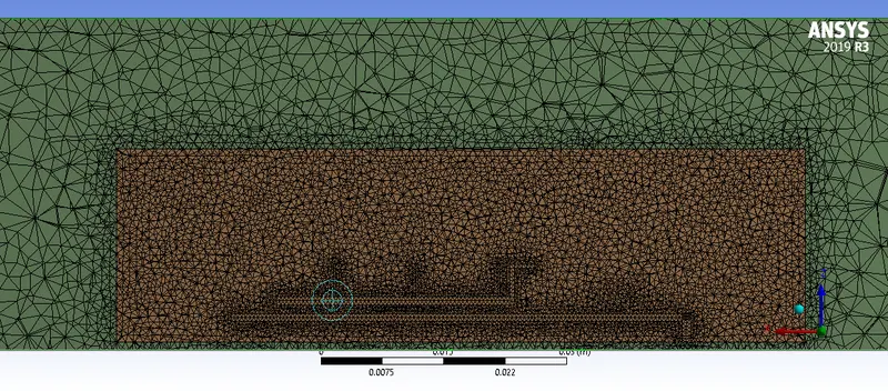
Mesh

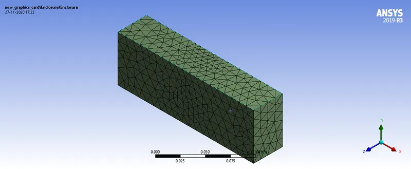
Mesh 1 - Automatically generated

Enclosure

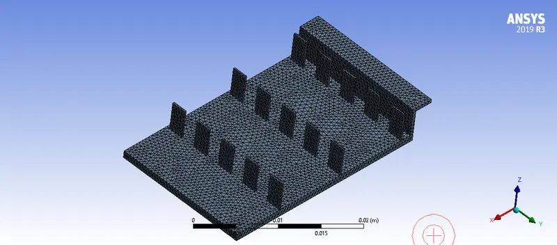
Graphics card

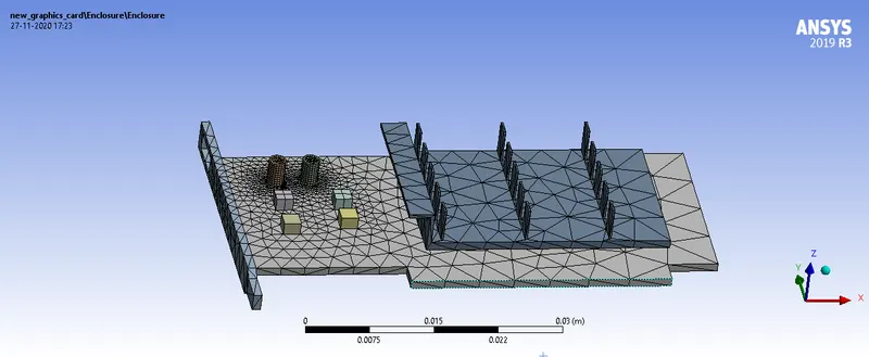
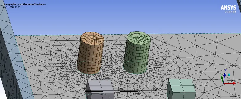
Near capacitor

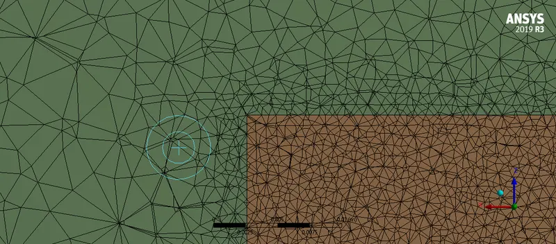
Mesh 2 - Refined

Outer Enclosure - Element size - 2.5 mm

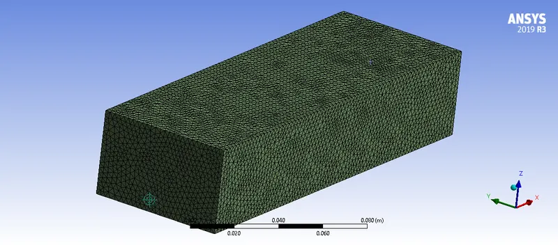
Inner Enclosure - Element Size - 1 mm

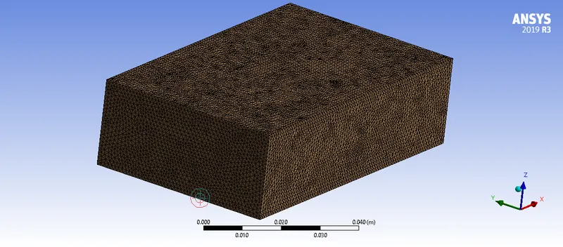
Interference of two meshes

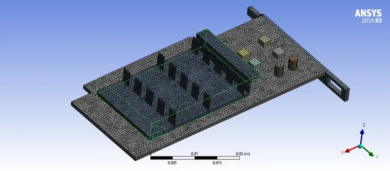
Graphics Card - Face sizing - 5mm

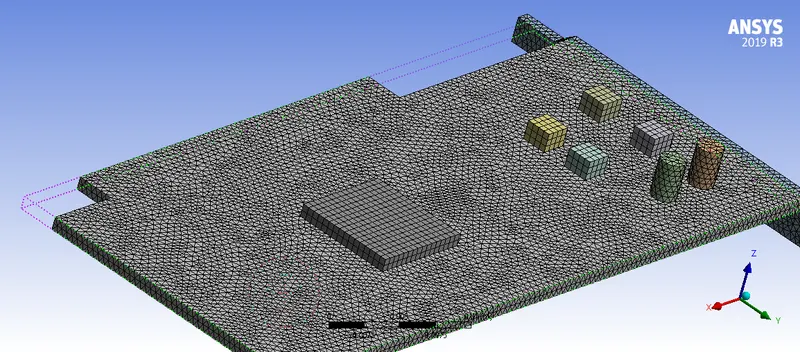
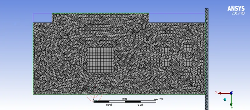
Near capacitor

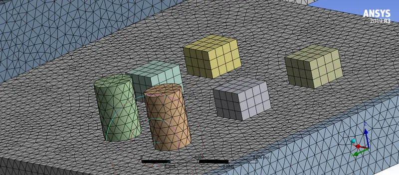
Fins

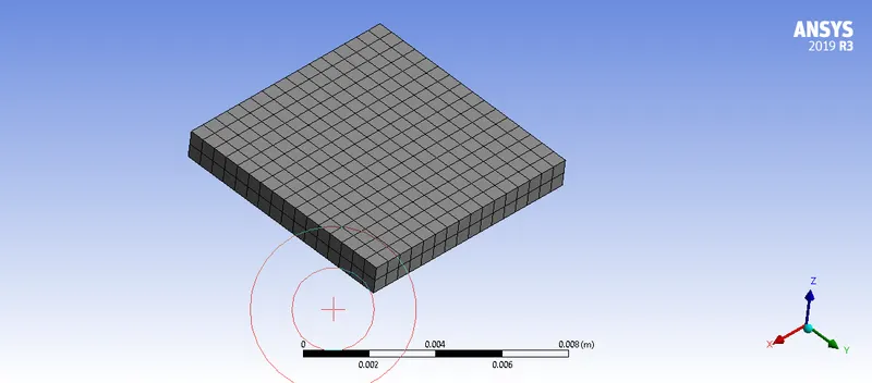
Processor

Mesh Statics

Mesh Metric - Aspect Ratio

Mesh Metric - Skewness

Boundary Conditions

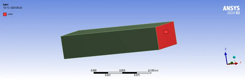
Inlet - Velocities - 1,3,5 `ms^-1`

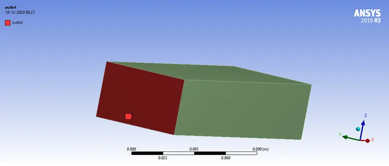
Outlet

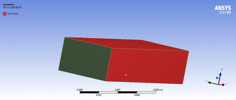
Symmetry

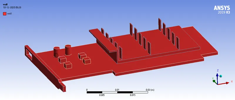
Wall

Solver Settings

Pressure Based - Steady State - solver was used

The processor was added a source term producing 156250000 `Wm^-3`

k -`omega` model with SST was used, even if the flow is laminar it will omit the turbulent terms and will act accordingly.

The energy equation was turned on as we need to calculate the temperature distribution.

Results :

For Mesh 1

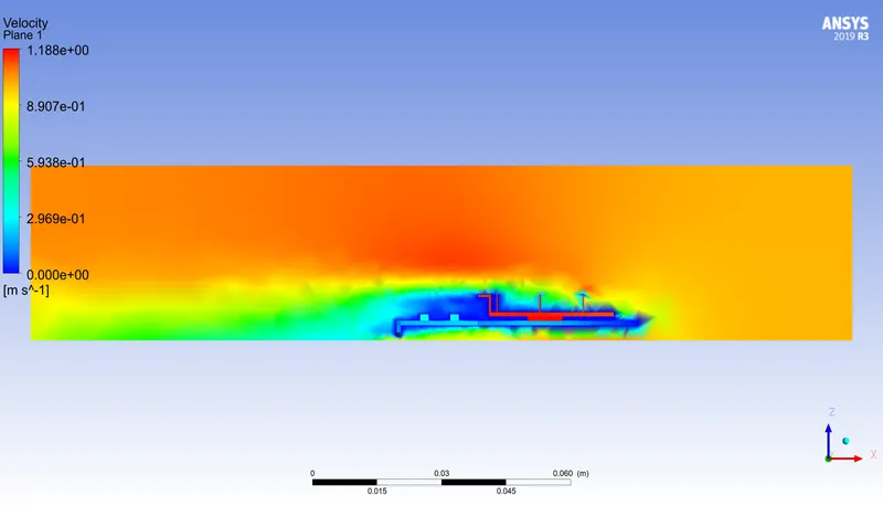
Every property is being compared for three velocities 1,3,5 `ms^-1` respectively

Residuals

In every case, a particular pattern started repeating itself and hence the convergence is achieved

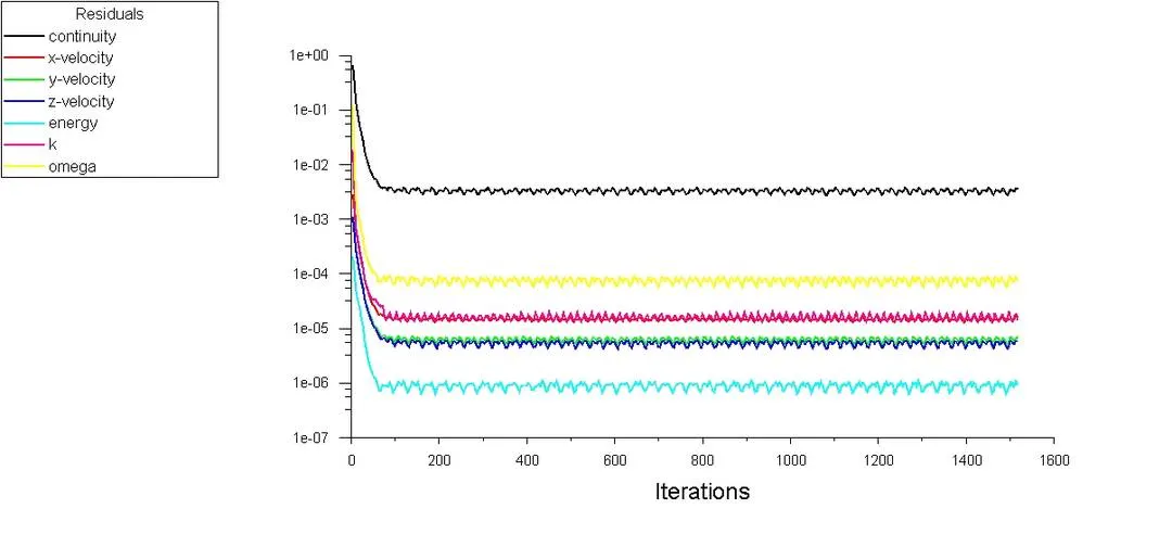
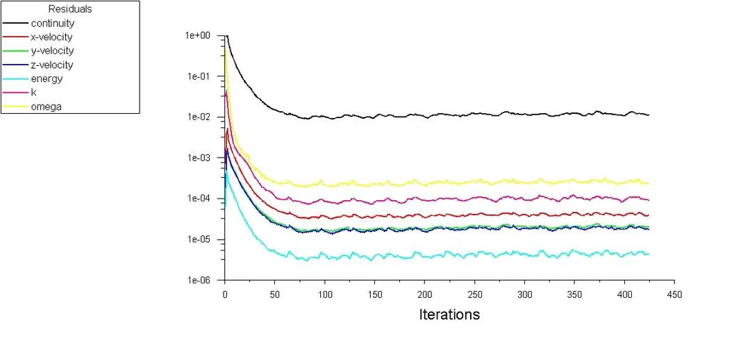
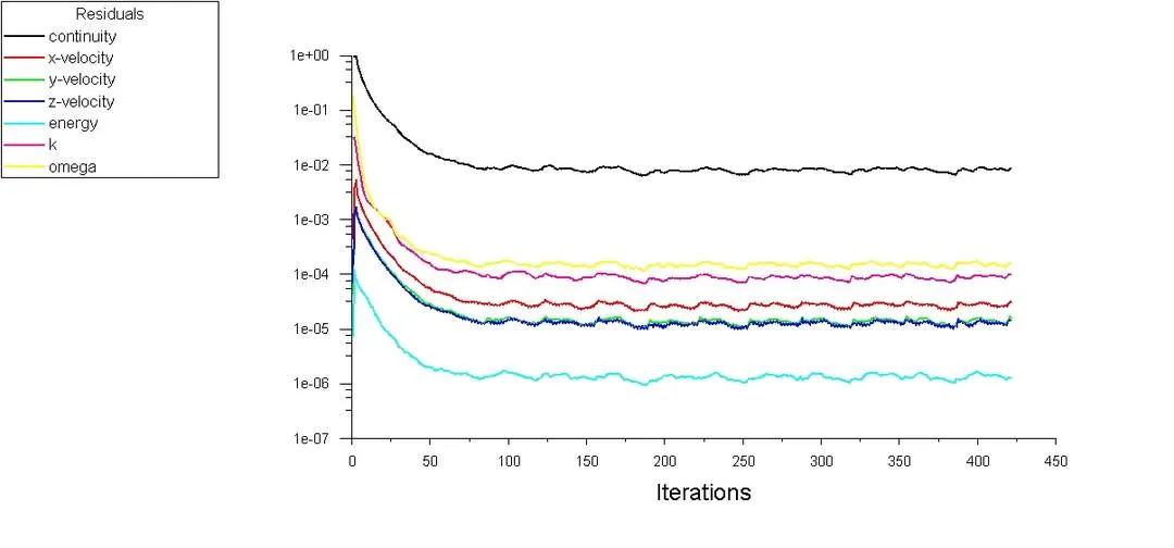
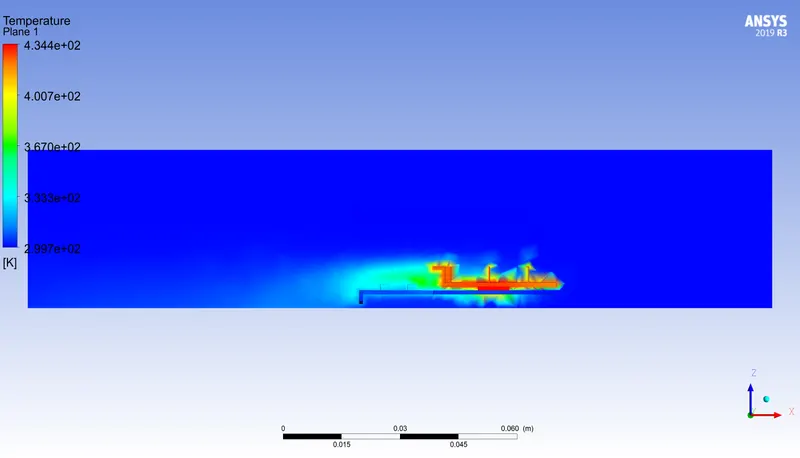
Temperature

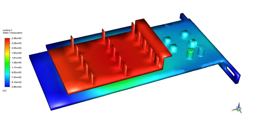
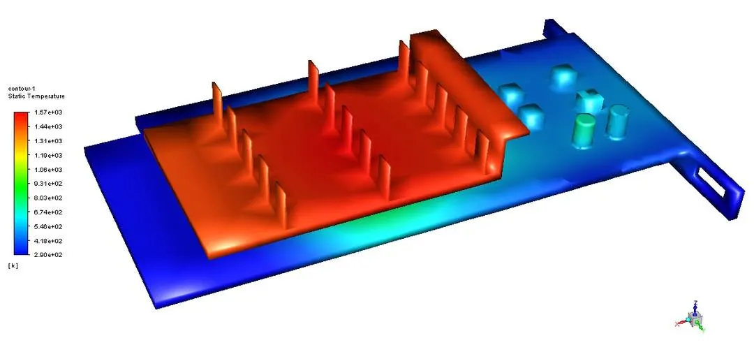
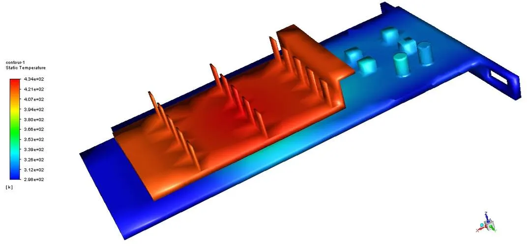
Temperature on the plane along with Graphics card

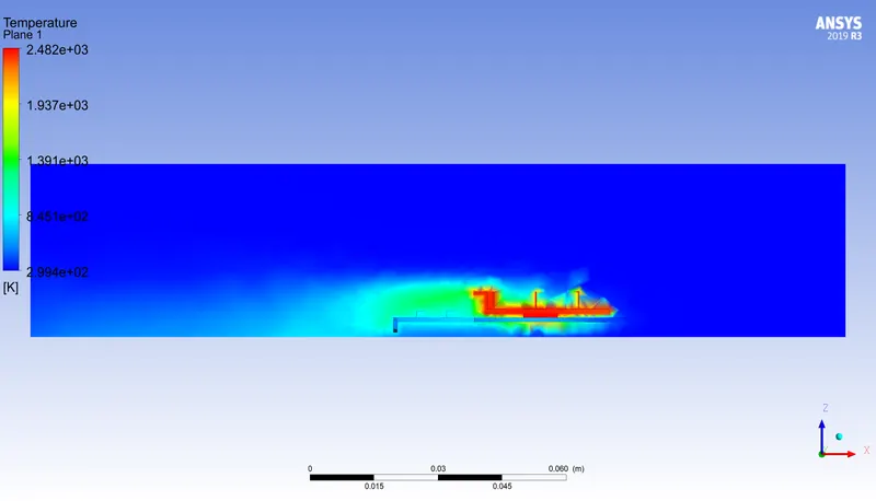
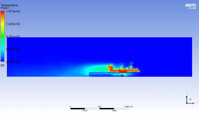
Velocity on the plane with the graphics card in temperature

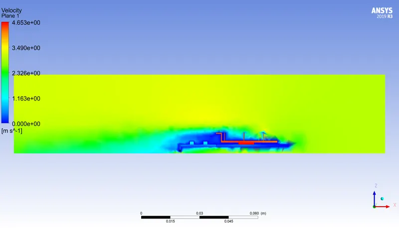
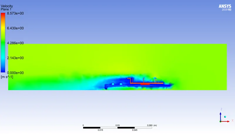
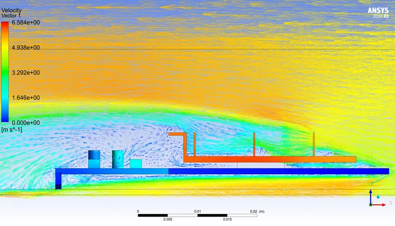
Velocity Vector

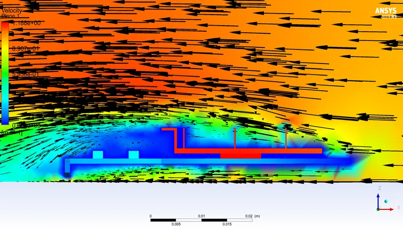
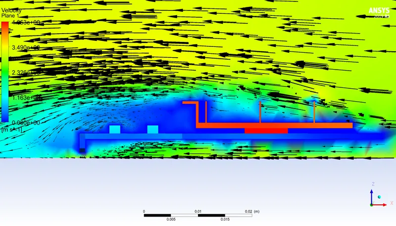
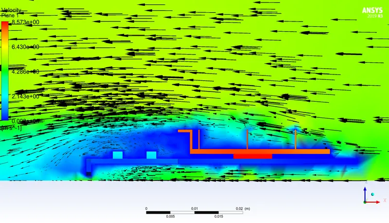
For Mesh 2

Every property is being compared for three velocities 1,3,5 `ms^-1` respectively

Residuals

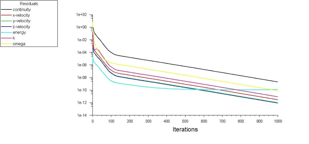
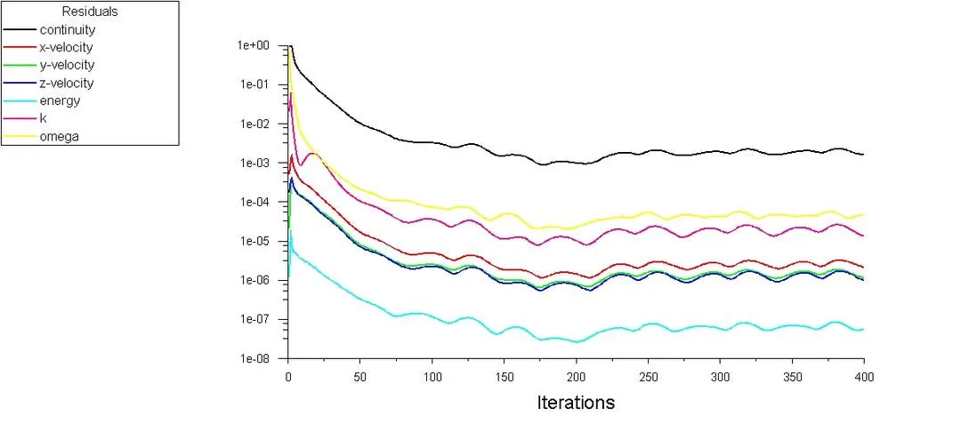
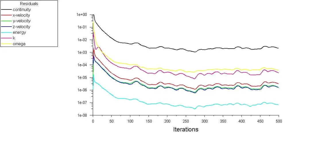
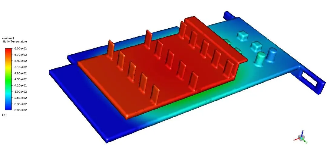
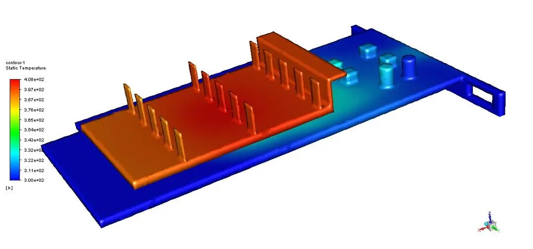
Temperature (static) distribution on graphics card

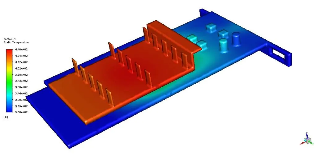
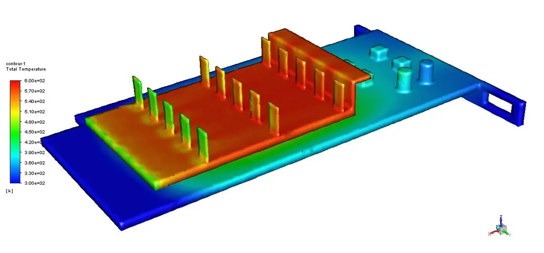
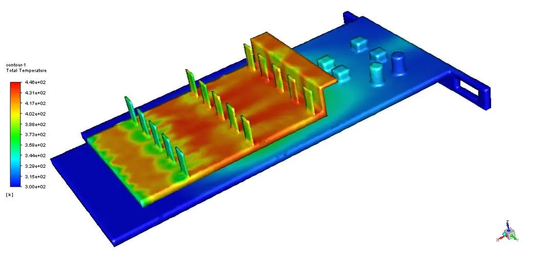
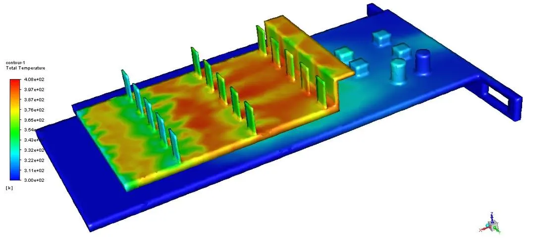
Temperature (total) distribution on graphics card

Temperature on plane and graphics card

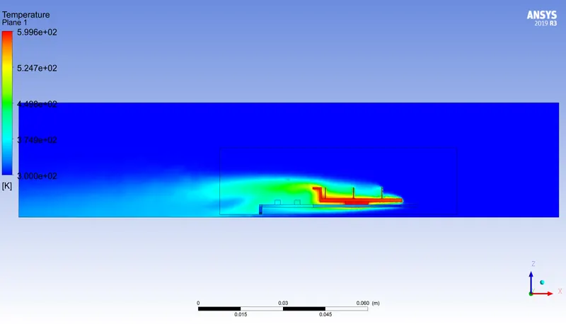
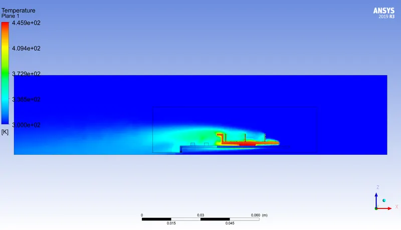
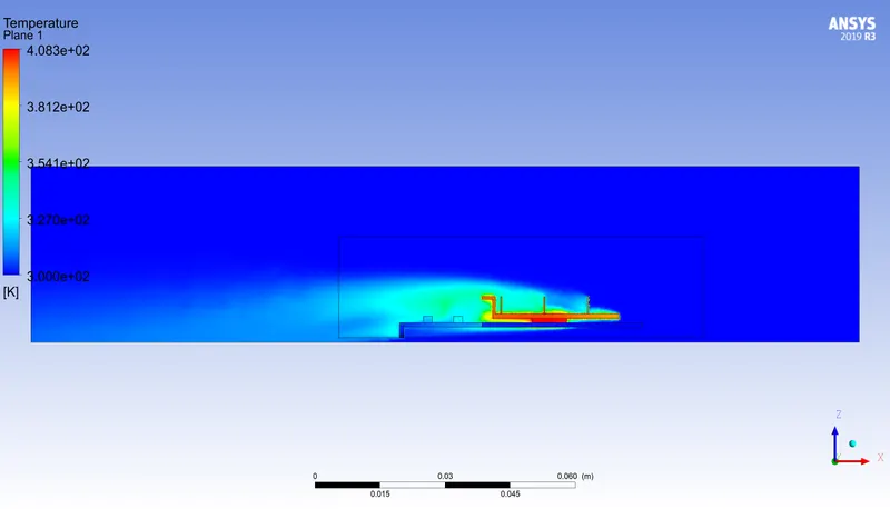
Velocity on plane and temperature on graphics card

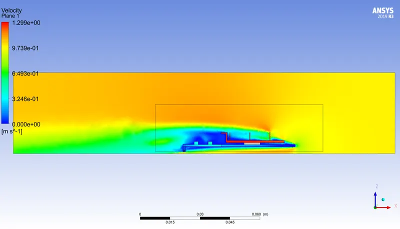
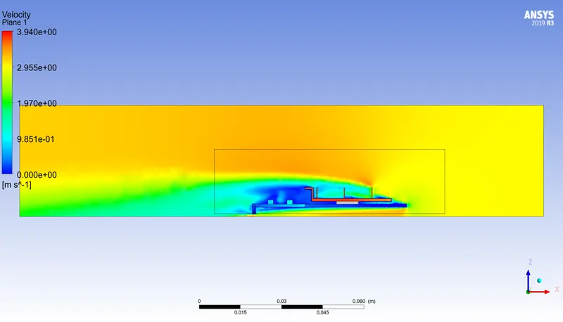
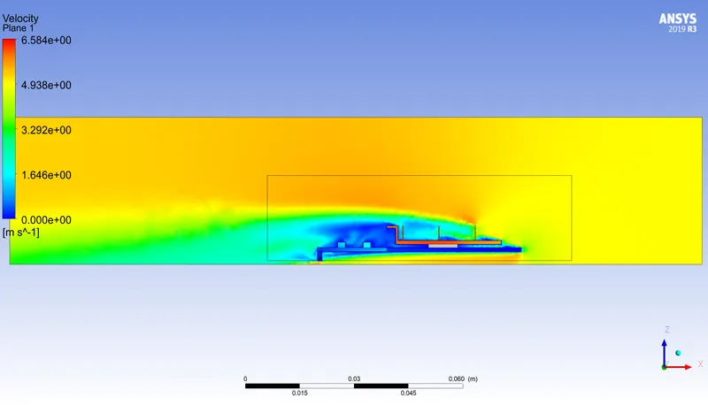
Velocity Vector

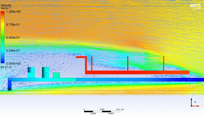
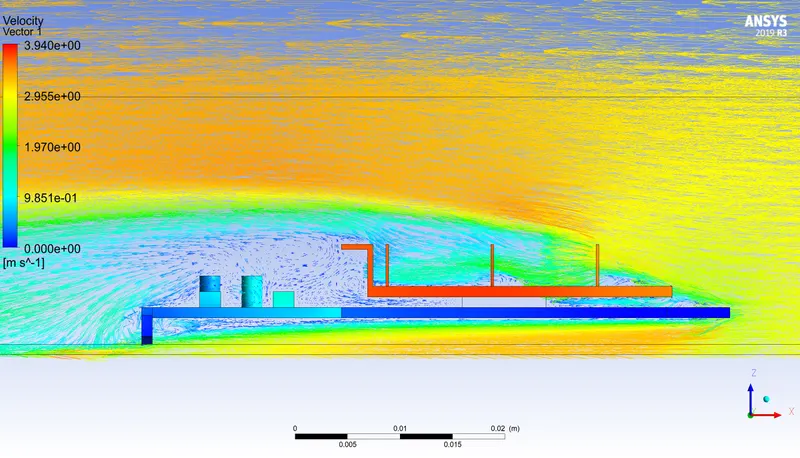
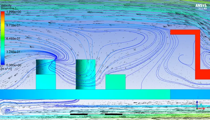
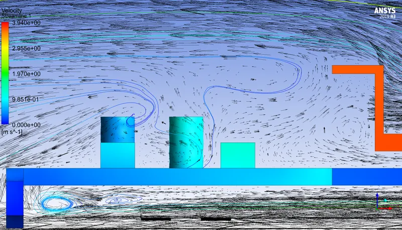
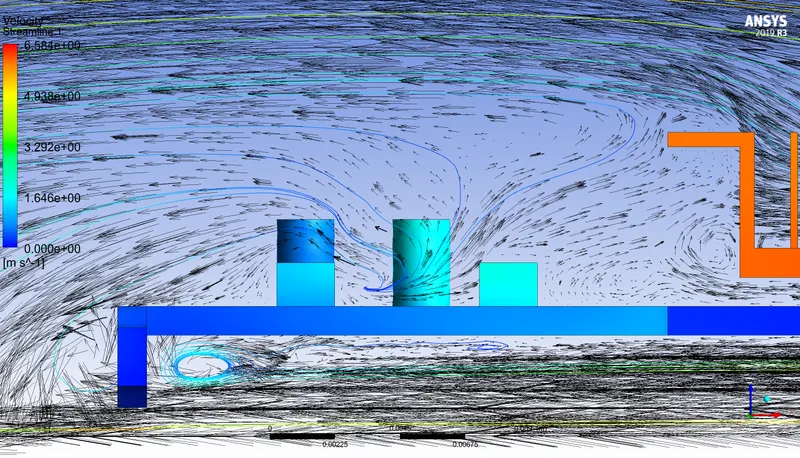
Velocity streamline with vector near capacitor

Temperature Distribution over board

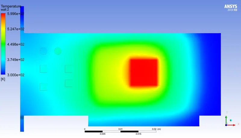
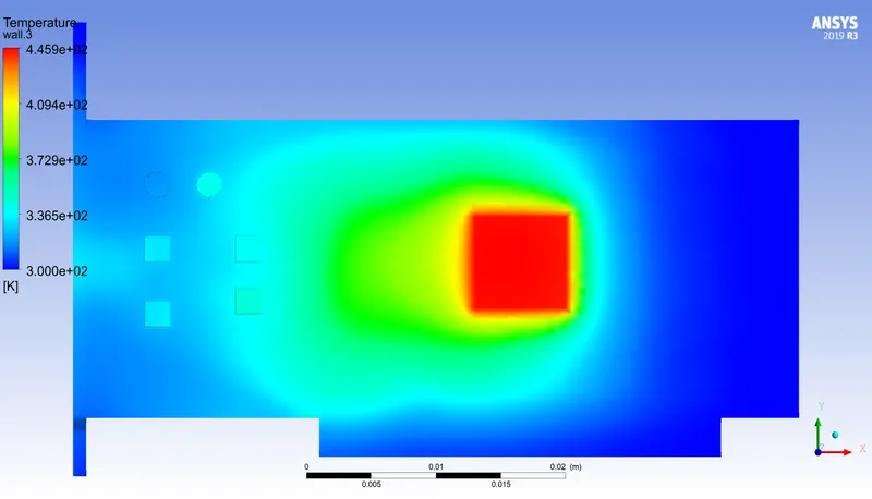
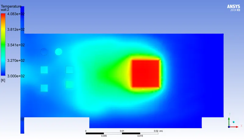
Temperature Distribution over board on back-side

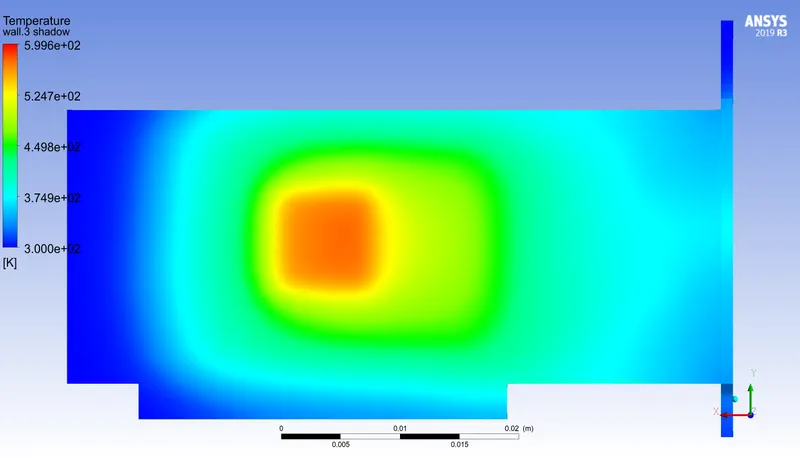
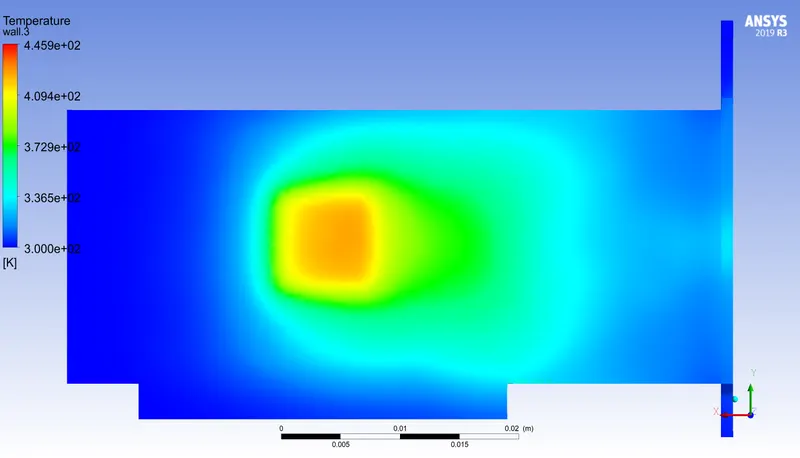
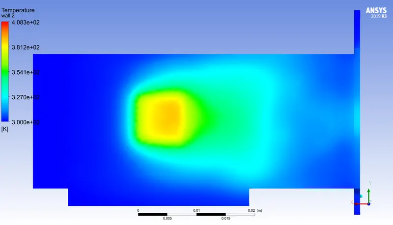
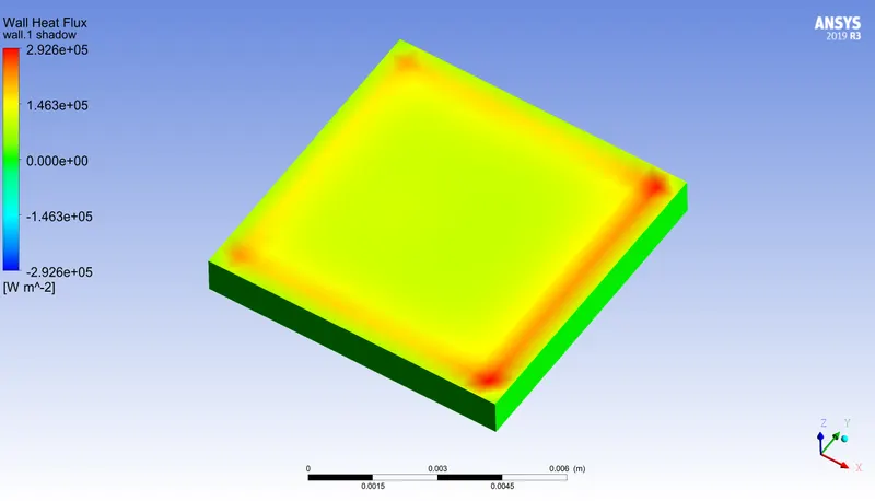
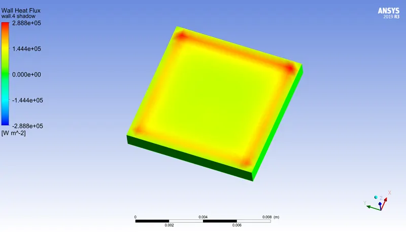
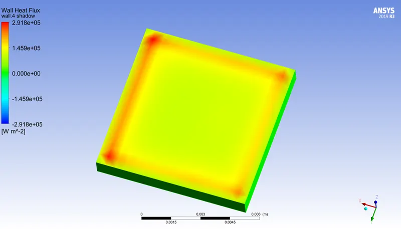
Heat flux from the processor

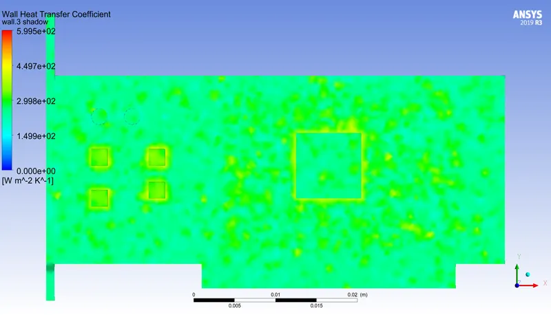
Heat transfer coefficient over the board

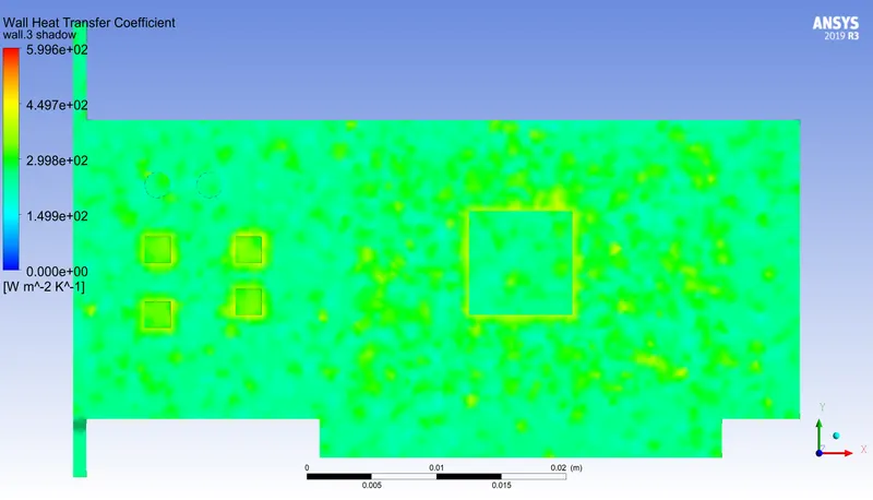
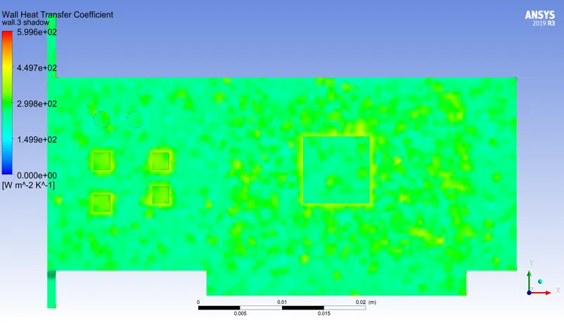
Heat transfer coefficient over Fins

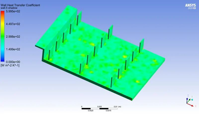
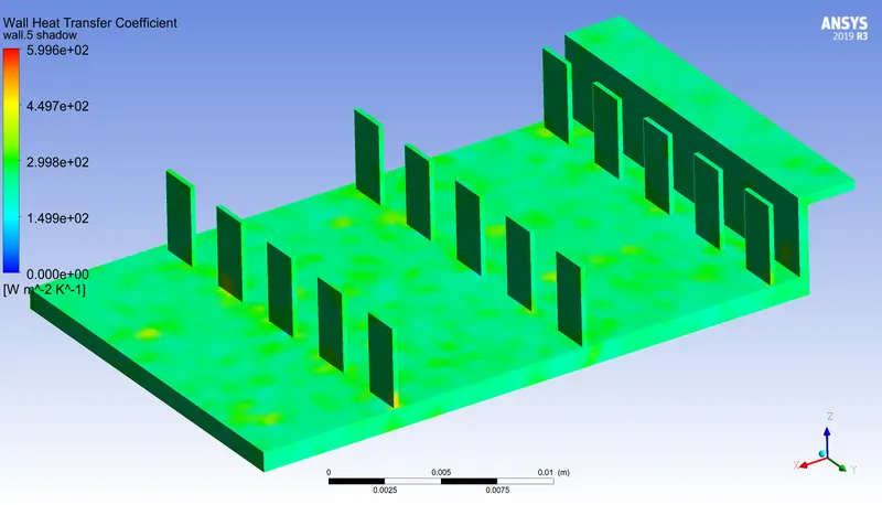
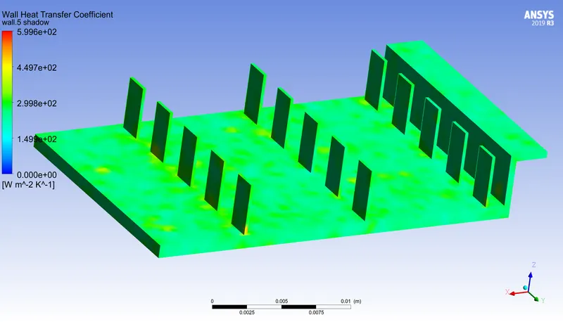
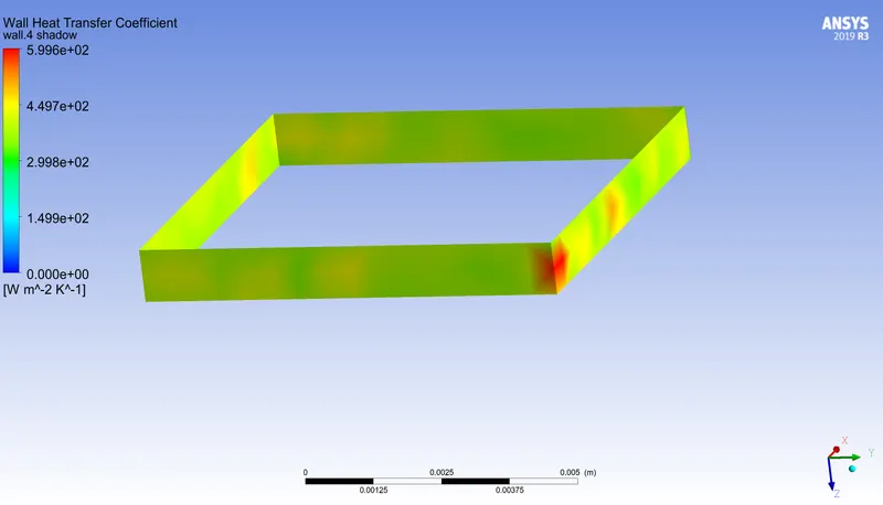
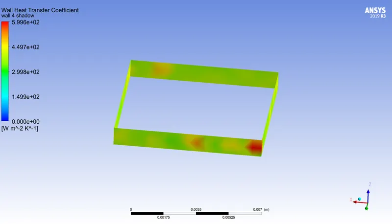
Heat Transfer Coefficient for Processor

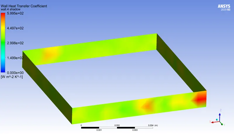
Animation of velocity vectors over graphics card

Heat Transfer Coefficient and Maximum Temperature for Processor

Velocity `(ms^-1)`	Heat Transfer Coefficient	Maximum Temperature (K)
1	5.996	600
3	5.996	446
5	5.996	405

Conclusions

1. It was observed that the higher the Velocity of flow more will be the cooling.
2. A coarse mesh can give highly inaccurate solution which may differ significantly from experimentation.
3. There were reverse flows in many cases.
4. In each case maximum velocity is more than the inlet velocity, it may be because of the heat absorption from the processor, which leads to rise in Kinetic energy

References

• Perelman, T. L. (1961). "On conjugated problems of heat transfer". International Journal of Heat and Mass Transfer.
• Luikov, A. V.; Perelman, T. L.; Levitin, R. S.; Gdalevich, L. B. (1971). "Heat transfer from a plate in a compressible gas flow". International Journal of Heat and Mass Transfer.
• https://www.nvidia.com/en-in/geforce/graphics-cards/gtx-1650/
• https://www.engineering.com/Hardware/ArticleID/17668/What-Raw-Materials-Are-Used-to-Make-Hardware-in-Computing-Devices.aspx#:~:text=GPUs%20are%20silicon%20layered%20with,cobalt%2C%20tungsten%2C%20for%20starter.