Rayleigh Taylor Instability Challenge

Aim

To perform and analyze Rayleigh Taylor instability for different conditions with different fluid

Introduction

Actually, The Rayleigh–Taylor instability, or RT instability, is the instability of an interface between two fluids of different densities which occurs when the lighter fluid is pushing the heavier fluid and can be observed in nature such as cloud formation after a volcanic eruption, nuclear explosion, and supernovas.

Theory

Water suspended atop oil is an everyday example of Rayleigh–Taylor instability, and it may be modeled by two completely plane-parallel layers of immiscible fluid, the denser on top of the less dense one and both subject to the Earth's gravity. The equilibrium here is unstable to any perturbations or disturbances of the interface: if a parcel of heavier fluid is displaced downward with an equal volume of lighter fluid displaced upwards, the potential energy of the configuration is lower than the initial state. Thus the disturbance will grow and lead to a further release of potential energy, as the more dense material moves down under the (effective) gravitational field, and the less dense material is further displaced upwards. This was the set-up as studied by Lord Rayleigh.

As the RT instability develops, the initial perturbations progress from a linear growth phase into a non-linear growth phase, eventually developing "plumes" flowing upwards (in the gravitational buoyancy sense) and "spikes" falling downwards. In the linear phase, the fluid movement can be closely approximated by linear equations, and the amplitude of perturbations is growing exponentially with time. In the non-linear phase, perturbation amplitude is too large for a linear approximation, and non-linear equations are required to describe fluid motions

Solving & Modelling approach

In the year 1883 Lord Rayleigh published a research paper "Investigation of the Character of the Equilibrium of an Incompressible Heavy Fluid of Variable Density", which dealt with the instability of junction of two fluid surfaces, in which fluid was arranged in horizontal strata and its density was represented by `sigma`, and change in density as `rho`, in which `rho` of the fluids at any point is a function of `(x,y,z,t)` and flow is considered as at very small velocity. The pressure was assumed as a function of `z` only, and variable pressure as `p + deltap`

and thus Governing equations take the form of :

`nabla.vecV = 0`

`(ddeltap)/(dx) = -sigma*(du)/(dt)`

`(ddeltap)/(dy) = -sigma*(dv)/(dt)`

`(ddeltap)/(dz) =-g*rho -sigma*(dw)/(dt)`

`(drho)/(dt) + w*(dsigma)/(dz) = 0`

analytical solutions of these equations appeared to be very complex and they can also be solved with numerical solutions

Pre-processing and solver setting

Geometry

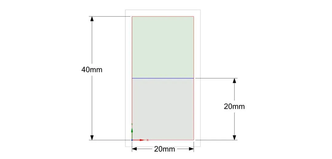
For geometry a rectangular plate with side 40 by 20 mm plate was used split in half, resulting in the square of side 20 mm and was prepared by SpaceClaim

Mesh

There were three meshes was used with different refinement status

Mesh 1 - Element size = 0.5 mm

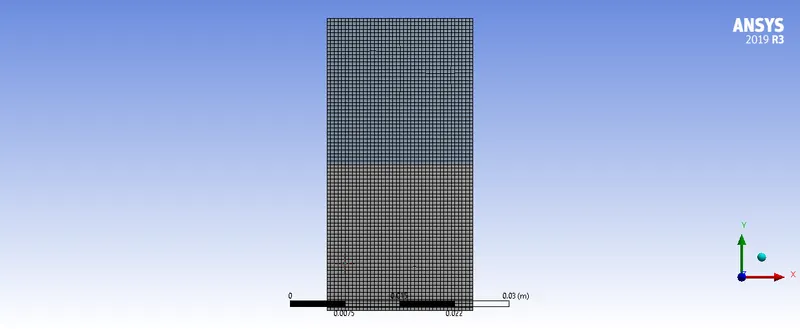
Mesh 2 - Element size = 0.25 mm

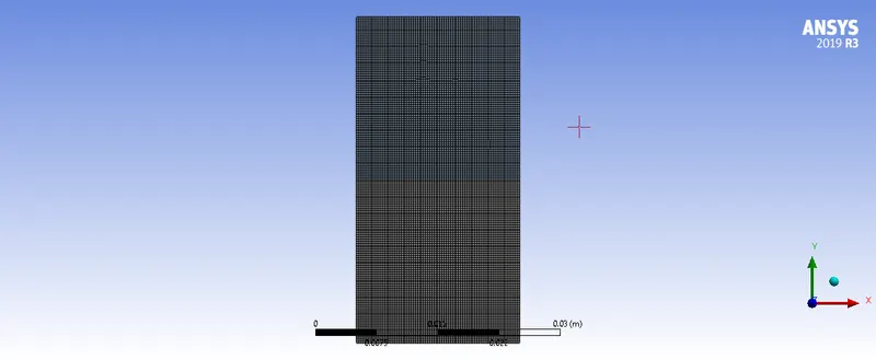
Mesh 3 - Element Size = 0.1 mm

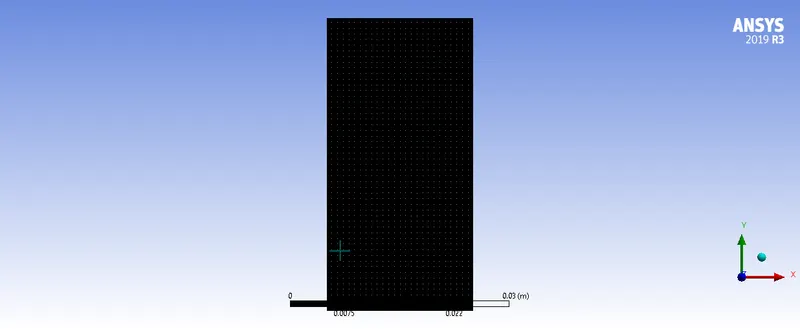
SOLVER

• As the velocity of fluids will be very slow Laminar model was used
• In the Multiphase Model, the Volume of Fluid method was used with the implicit formulation
• Patching was done after Standard Initialisation
• Pressure based Transient solver was used
• And gravity was taken 9.81 `ms^-2` in the negative y-direction

Steps

1. A total of four simulations was performed
2. Out of which three were performed between water and air
3. The last simulation was performed between water and user-defined fluid along with the Mesh 3 as it is the most refined

User Defined Fluid

Density	400
Viscosity	0.001

Results

Residuals

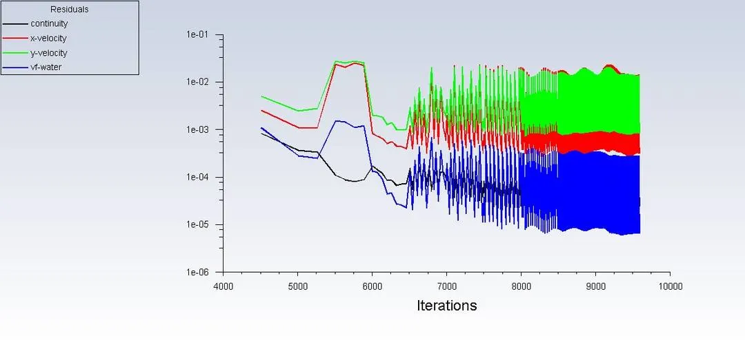
Simulation 1 - Mesh 1 - Water vs Air - Step Size 0.005s

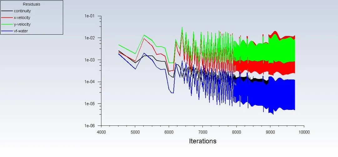
Simulation 2 - Mesh 2 - Water vs Air - Step Size - 0.005s

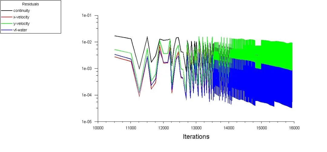
Simulation 3 - Mesh 3 - Water vs Air- Step Size - 0.003s

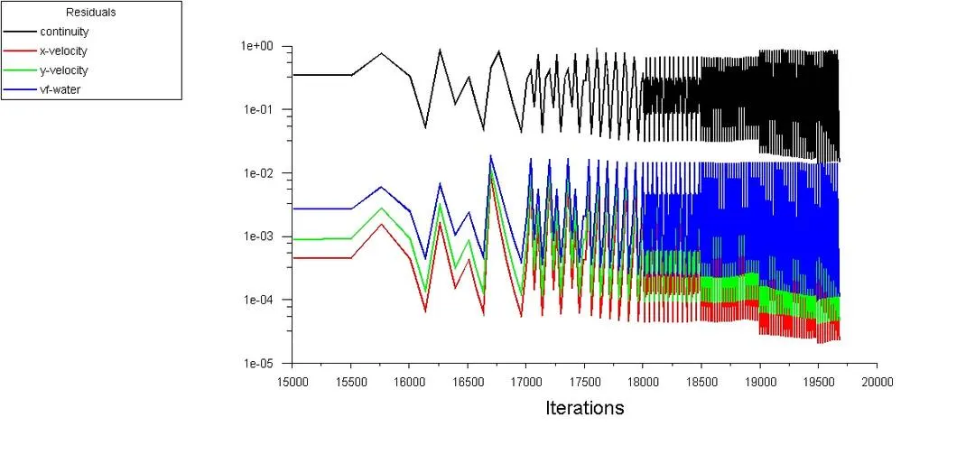
Simulation 4 - Mesh 3 - Water vs User-Defined Fluid - Step Size - 0.003s

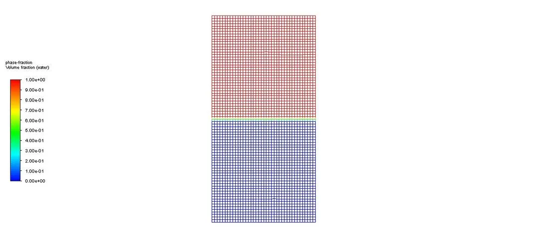
For every simulation just before mixing fraction contour

Water - (Red)

Other Fluid - (Blue)

Simulation Videos

Simulation 1

Simulation 2

Simulation 3

Simulation 4

Atwood Number

The Atwood number (A) is a dimensionless number in fluid dynamics used in the study of hydrodynamic instabilities in density stratified flows. It is a dimensionless density ratio defined as

A = `(rho_1-rho_2)/(rho_1 + rho_2)`

`rho_1` = density of the heavier fluid

`rho_2` = density of lighter fluid

Material	Density
Water	1000
Air	1.225
User-Defined fluid	400

Simulation No	Atwood Number
Simulation 1,2,3	0.9975
Simulation 4	0.4285

Conclusion

• It was observed that more refined mesh gives a more realistic simulation
• It was observed that more viscosity leads to more time in getting settled
• The higher the Atwood Number higher will be the penetration by heavier liquid

References

1. Rayleigh, Lord (John William Strutt) (1883). "Investigation of the character of the equilibrium of an incompressible heavy fluid of variable density". Proceedings of the London Mathematical Society. 14: 170–177
2. Drazin, P. G.; Reid, W. H. (2004). Hydrodynamic stability (2nd ed.). Cambridge: Cambridge University Press
3. Grove, J. W.; Li, X.-L.; Oh, W.; Sharp, D. H. (2001). "A critical analysis of Rayleigh–Taylor growth rates"