Steady Vs Unsteady flow over a cylinder

Aim

1. To simulate the flow with the steady and unsteady case and calculate the Strouhal Number for Re= 100.
2. To calculate the coefficient of drag and lift over a cylinder by setting the Reynolds number to 10,100,1000,10000 & 100000 using steady-state solver
3. To discuss the effect of Reynolds number on the coefficient of drag

Introduction

Fluid Mechanics is one of the most fascinating topics of Physics, and it is most beautiful when we are trying to experiment things and making conclusion out of them, so here we are trying to simulate the flow past cylinder problem

Flow past over a cylinder is one of the most famous and effective experiments in the world of fluid dynamics and has wide application in the field of aerodynamics to everyday fluid machines and natural fluid mechanics phenomena. Here we are trying to simulate flow over such a case for different parameters to see the nature of the flow.

Theory

When we put a cylinder on the stream of water(or any fluid), there are lots of fluid mechanical phenomenon which results in many different types of experimental results and some of them is shown in the picture below

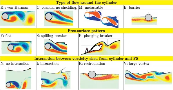
Here we will try to understand the Von Karman Vortex

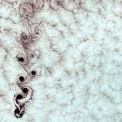
Von Karman Vortex formation due to an island’s mountain top, acting as an obstacle in the path of air and cloud

To understand Von Karman vortex shedding, we first need to understand the concept of vortex shedding.

Due to flow separation sometimes, there is a vortex generation, and the periodic generation of these vortices downstream is referred to as vortex shedding and this phenomenon usually occurs during normal flow over long cylinders or spheres for Reynolds number ≥ 90. These vortices can lead to serious vibration problems, and if their frequency of vibration gets equal to the natural frequency of our body or desired device and machine, it can lead to disaster. Let the frequency of vibration is f and D be the diameter of our cylinder, and V is the flow velocity. By these parameters, we can define the Strouhal number, which is basically the ratio of oscillations to mean speed

`St = (fD)/V = (oscillation)/(mean speed)`

and von Karman vortex shedding is nothing but the repeating pattern of swirling vortices

The Strouhal number is a dimensionless number describing oscillating flow mechanisms and named after Czech physicist Vincence Strouhal

Solving

In this study, we are going to vary Reynold’s number

`Re = (rhovd)/mu`

here transient solver was used with

Size of time step = 0.1s

Number of time steps = 1000

Geometry

For our domain of calculation and simulation, we are using the following geometry

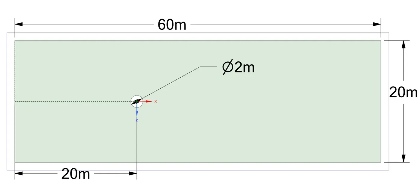
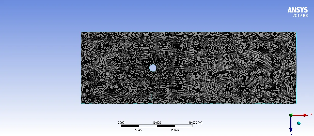
Here we will perform simulation on a cylinder of diameter D = 2m and the size of the complete domain is 60 by 20

And is in the shape of a rectangle

Meshing

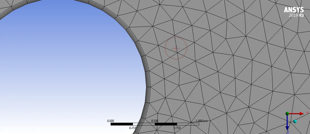
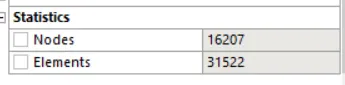
Here for meshing, we’ve preferred to triangular-shaped elements with element size = 0.025 and for more better result, we have divided the circumference of the cylinder into 36 parts

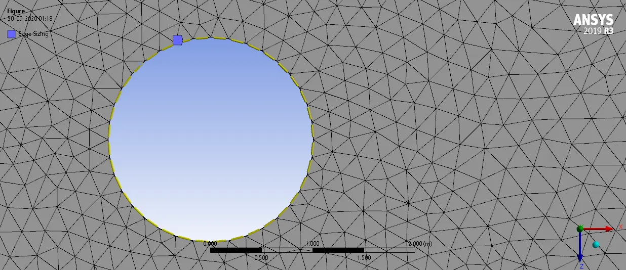
For better results, inflation was added with 6 layers and growth of 1.2 % with initial layer thickness 5e-03

Material

For simulation, we’ve used an imaginary fluid with the following properties

Density = 1

Viscosity = 0.02

Inlet Velocity = 1

this gives

`Re = 100`

Boundary Conditions

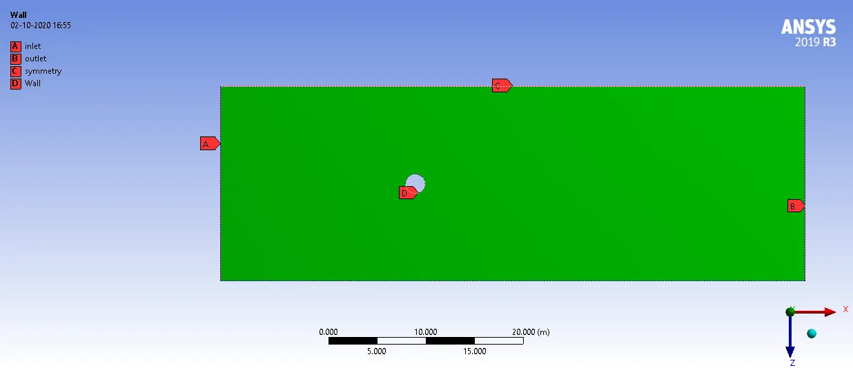
Inlet: Inlet surface is represented by `A` in the picture and here it is set to `1 ms^(-1)`

Outlet: Outler surface is represented by `B` in the picture and here it is pressure outlet and set to gauge pressure = 0

Wall: Wall is represented by `D` the surface of the cylinder in contact with the fluid as it will be at rest always, it's any kind of motion is set to zero

Symmetry: Symmetry is nothing but the symmetry of the domain

Now boundaries are named as :

Results

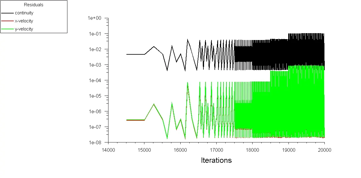
Convergence plot for Residuals

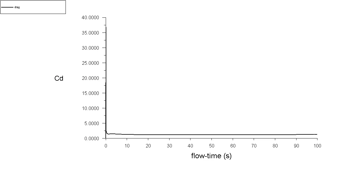
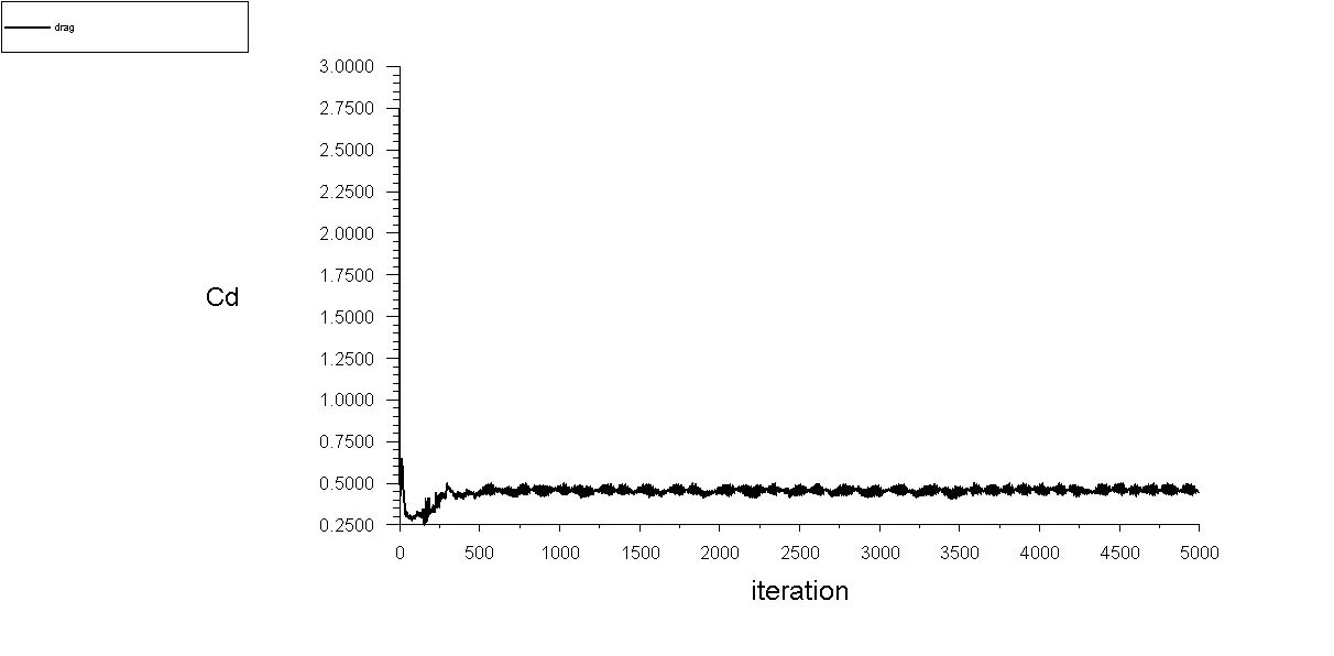
Coefficient of drag `C_(d)`

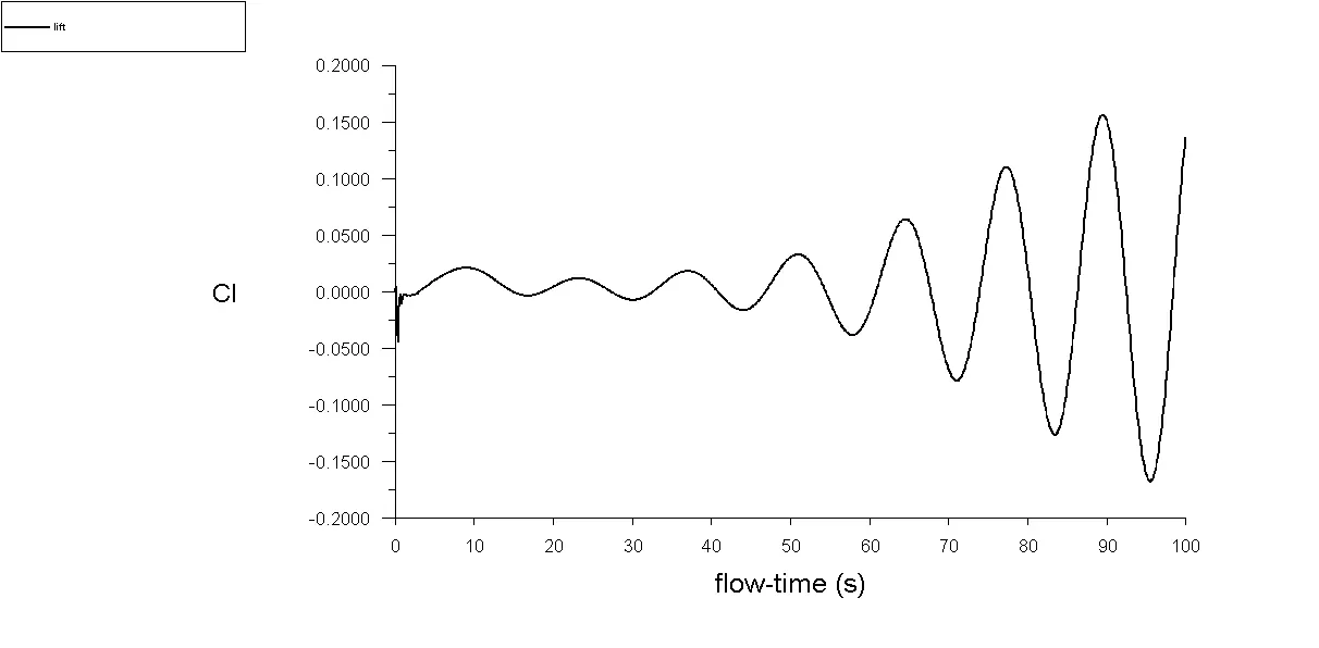
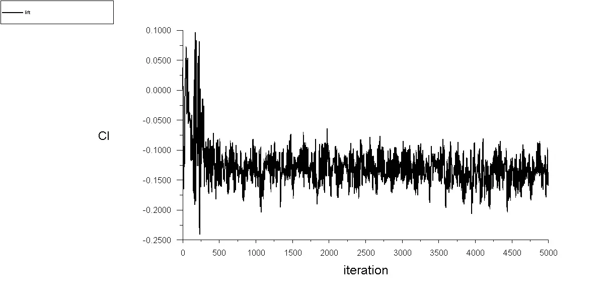
Coefficient of Lift `C_(l)`

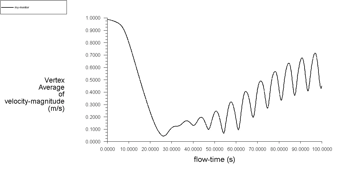
Velocity fluctuation at a point to the right of cylinder with X = 8m (horizontal distance) and Y(vertical distance) = 0

Countour of Velocity after the Von Karman Vortex shedding was established

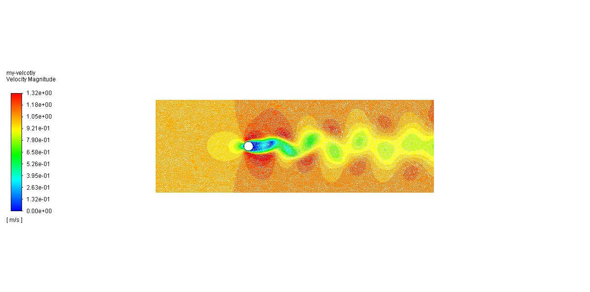
Animation

Strouhal Number

This graph was obtained in using FFT for Strouhal number, then all the data was exported to a different file and was analyzed in Excel

and the Strouhal number at which Magnitude is maximum will be the required number. In this case, it is 1.60e-01

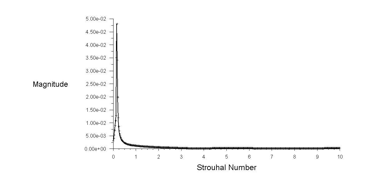
`St = (fD)/V = (oscillation)/(mean speed) `

`St = 0.16`

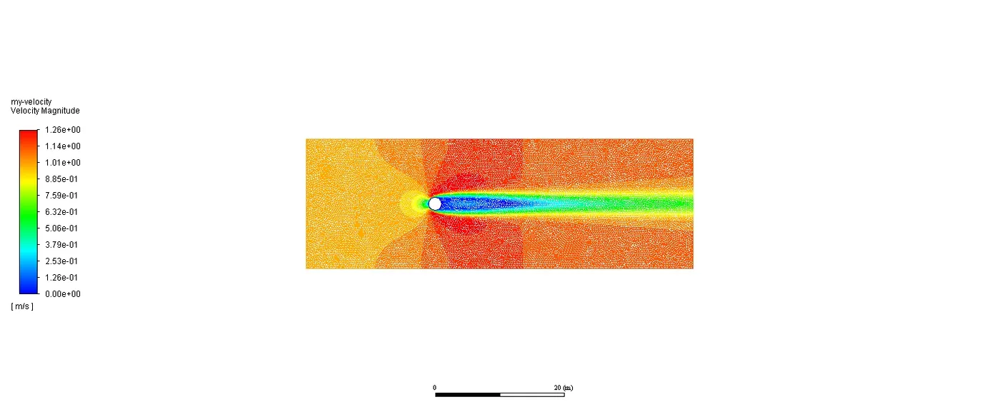
Results for Re 100 using Steady-State Solver

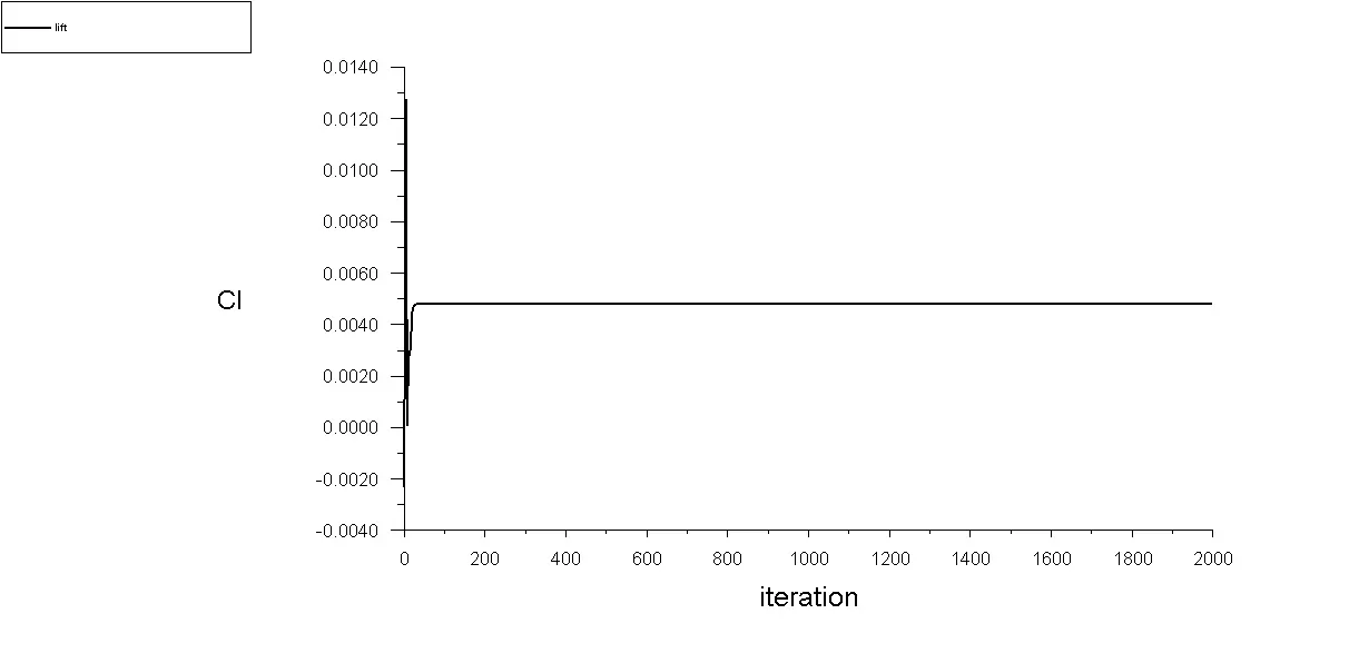
Total iterations = 2000

Convergence of residuals

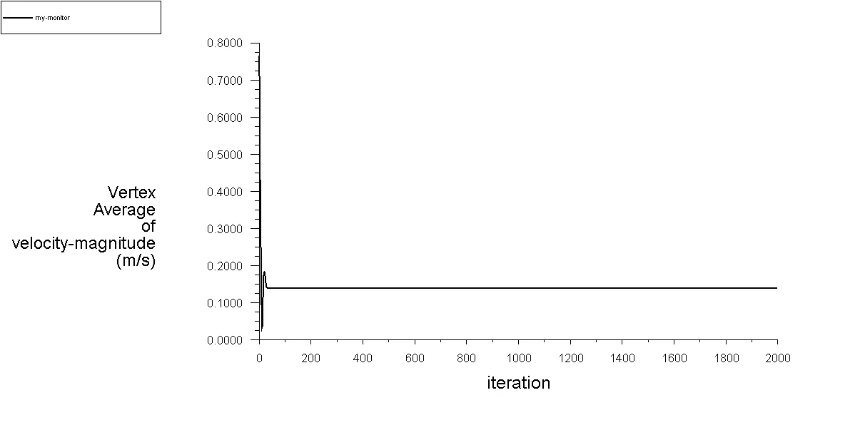
Plot of Cd

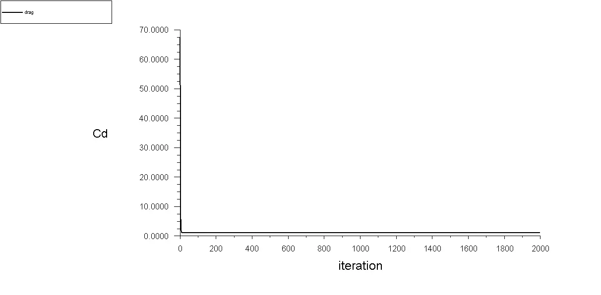
Plot of Cl

Contour Plot for Velocity

Part II: Solving using Steady-state solver

In this part above Cd and Cl will be calculated for Re = 10,1000,10000,100000 using Steady-State Solver

For different values of Re Velocity was varied by keeping all other terms constant

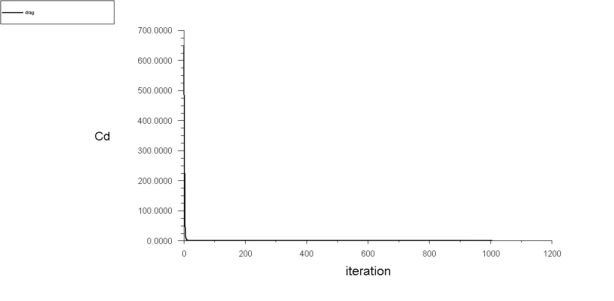
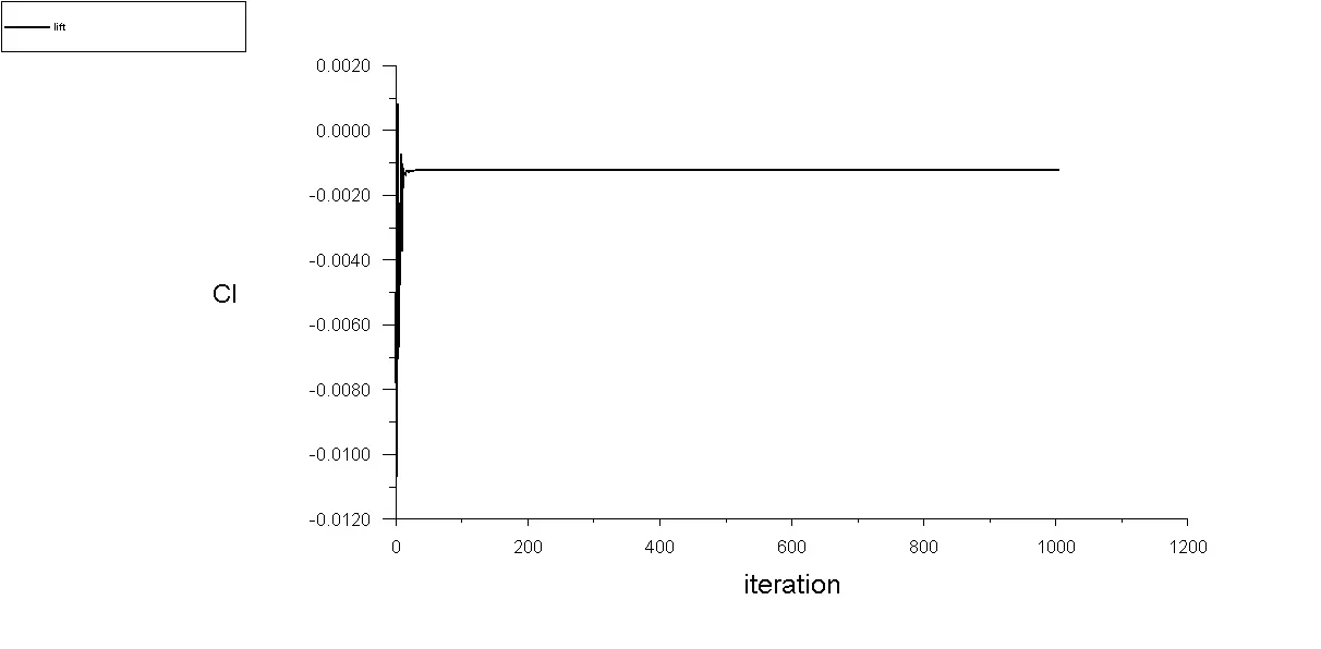
Re 10

PLOT FOR `C_(d) and C_(l)`

Re 1000

PLOT FOR `C_(d) and C_(l)`

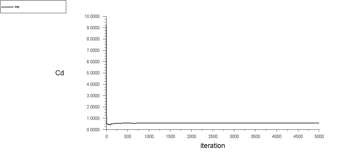
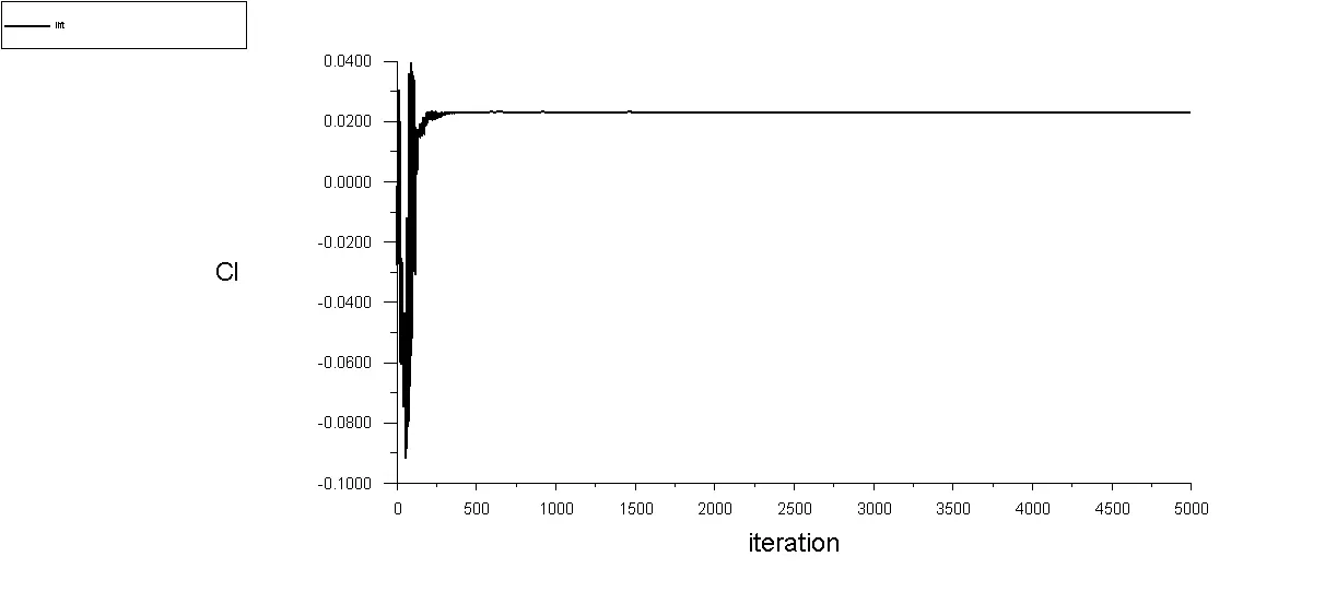
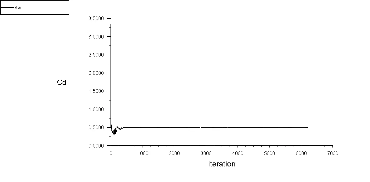
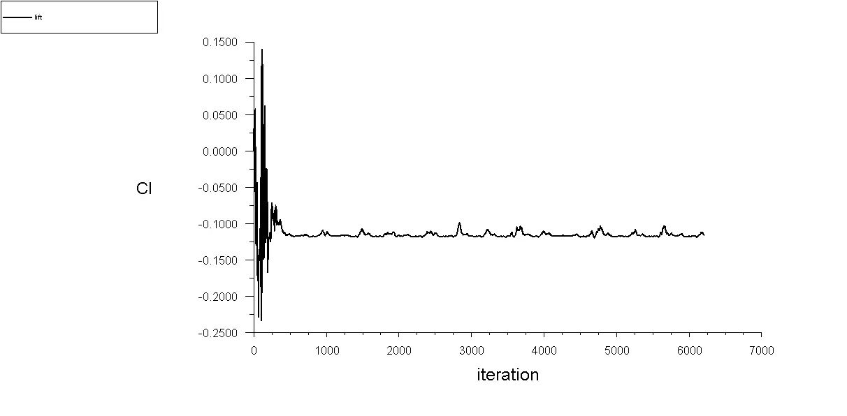
Re 10000

PLOT FOR `C_(d) and C_(l)`

Re 100000

PLOT FOR `C_(d) and C_(l)`

A tabular representation of `Re,V,C_(l),C_(d)`

Reynold’s number	Velocity	Drag coefficient	Lift Coefficient
10	0.1	3.3262103	0.0012079671
100	1	1.3560269	0.13735594
1000	10	0.5873316	0.023245186
10000	100	0.50635117	0.11470319
100000	1000	0.44897242	0.15141557

Material

Throughout the simulation project, a hypothetical fluid was used with the following properties :

`mu = 0.02`

`rho = 1`

and only the velocity was varied for obtaining different Reynold's Number

Conclusion

• It can be seen from the above table that on increasing Reynold's number, the drag coefficient tends to increase
• Variation of lift coefficient was random on varying Reynold's number
• It would better if we use transient-solver for solving transient process because they tend to give us a more accurate and far better result than a steady-state solver
• It was fun to see the velocity contour for different Reynold's number especially their animation

References

1. Fluid Mechanics 8th edition, Frank M. White
2. Fluid Mechanics: Fundamentals and Applications 3rd edition by John Cimbala and Yunus A. Cengel
3. http://hmf.enseeiht.fr/travaux/CD0102/travaux/optmfn/gpfmho/01-02/grp6/pages/strouhal.htm
4. SPH modeling of viscous flow past a circular cylinder interacting with a free surface by Benjamin Bouscasse, Andrea Colagrossi, Salvatore Marrone, Antonio Souto-Iglesias