Mixing efficiency
| Case | Case 1 (k epsilon - Realize) | Case 1 (k omega SST) | case 2 |
| Cell Count | 82108 | 82108 | 112932 |
|
Average outlet temperature |
36.473041 |
35.5 |
35.012425 |
|
Number of iterations for convergence |
163 | 950(approx) | 138 |
| Standard Deviation of Outlet Temperature | 3.18 | 3.15 | 2.81 |
So, clearly, in this case, both models have approximately the same Outlet Avg Temperature and Standard Deviation
But K omega is taking more time as well as more iterations as compared to K epsilon, hence for Case 2 we'll
use K - epsilon model with Realize
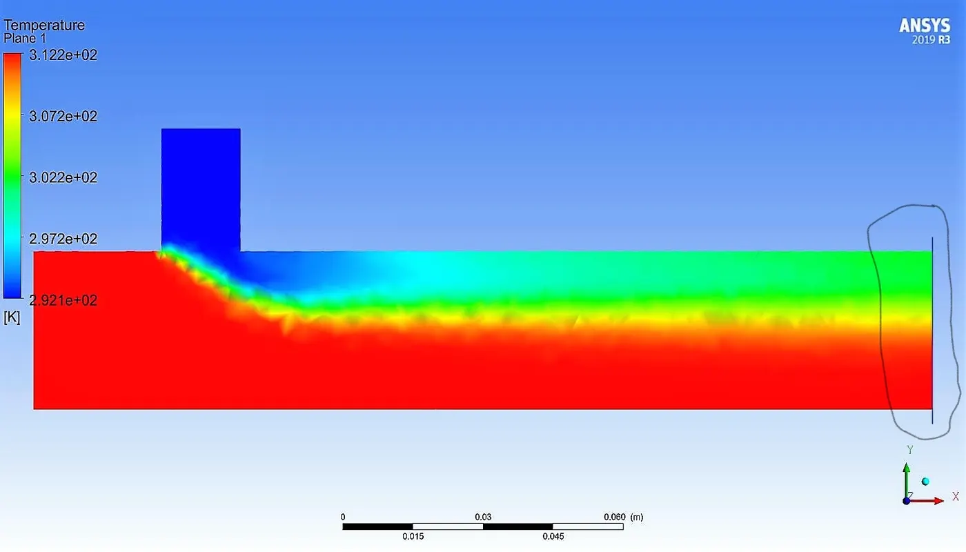
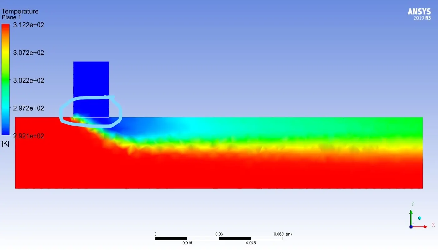
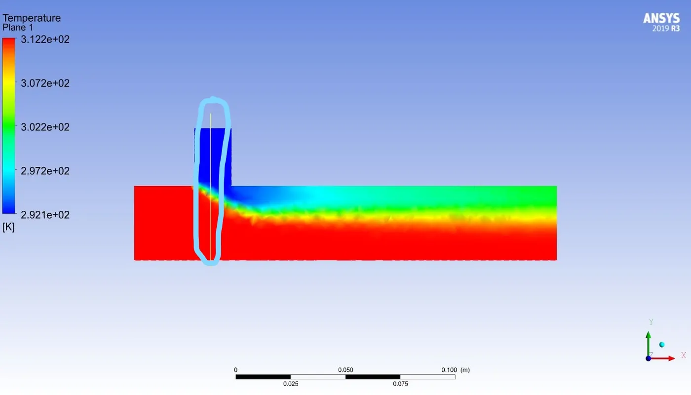
For Variation Across the pipe, these three positions are used:
1. Outlet Cross Section
2. Junction Cross Section along X
3. Along Cold Inlet
FOR CASE 1
Viscous effect - K epsilon model - Realize
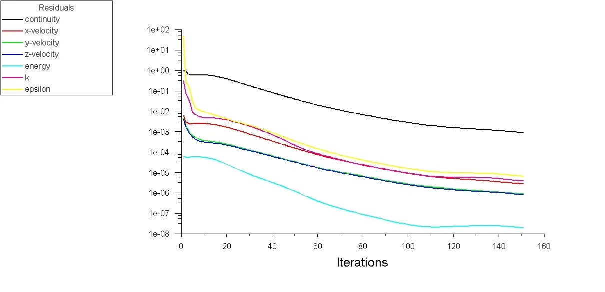
Convergence of Residual
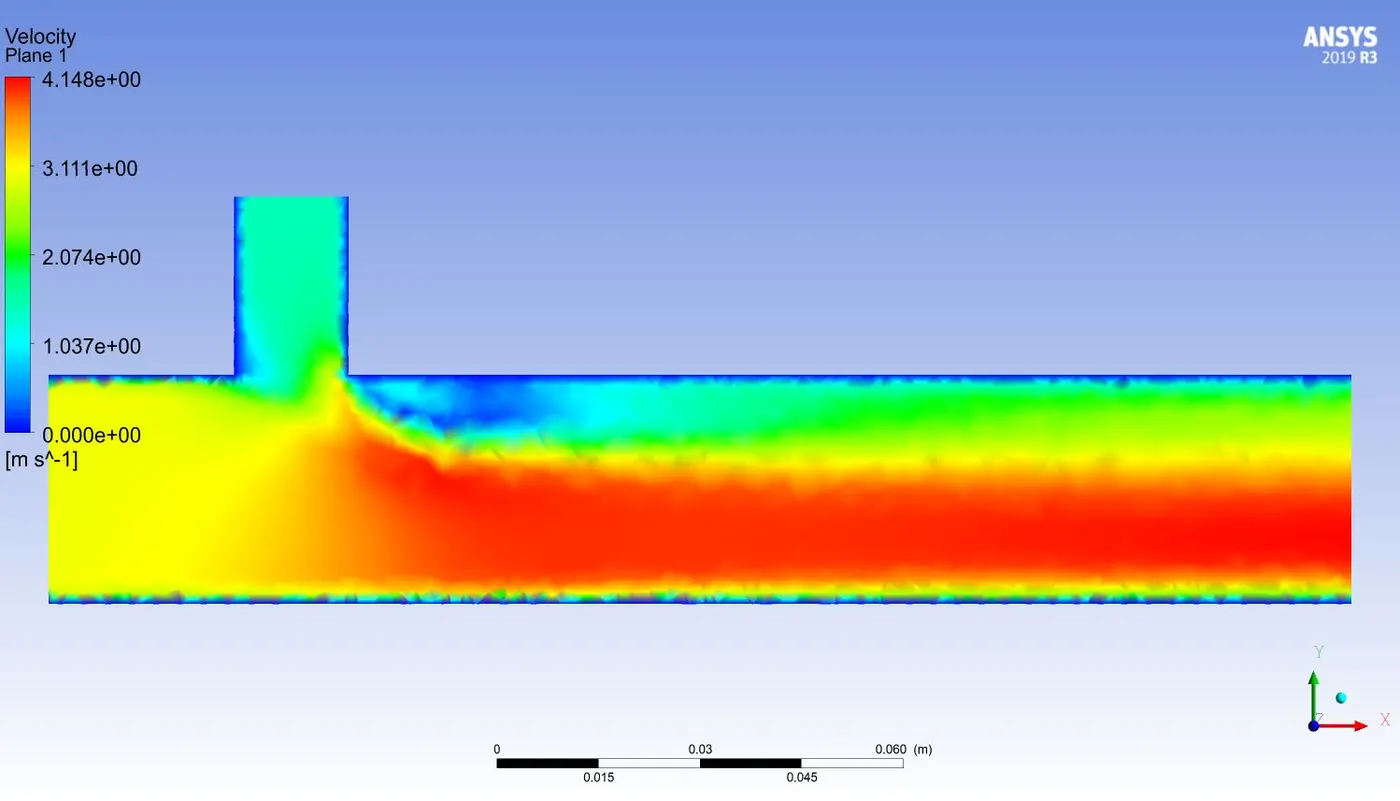
Resultant Velocity Variation on Plane
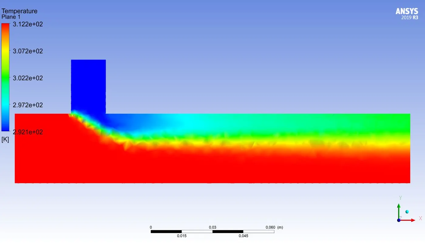
Temperature Variation in Plane
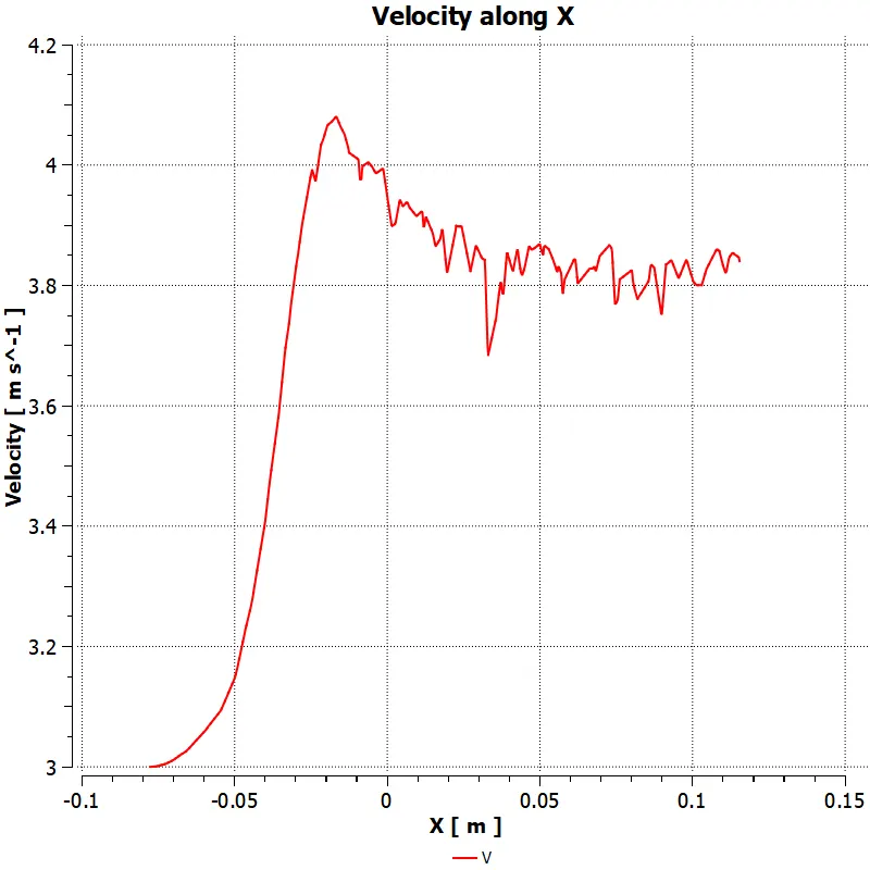
Velocity Variation along the length of pipe
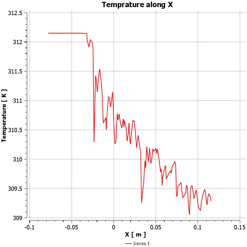
Temperature Variation along the length of pipe
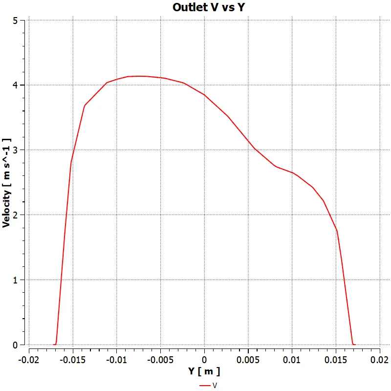
Velocity variation across the outlet
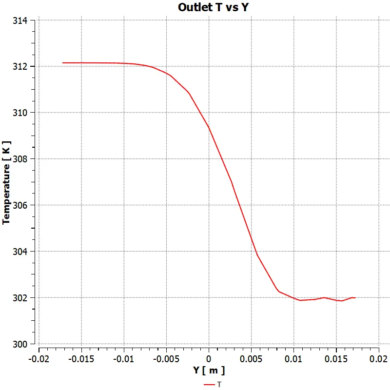
Temperature variation across the outlet
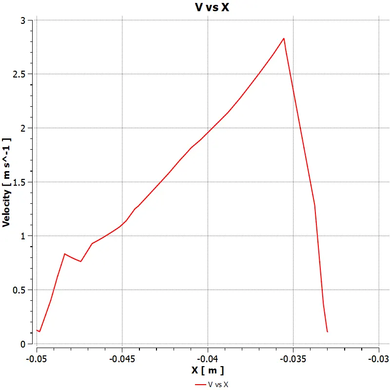
Velocity variation at Junction along X
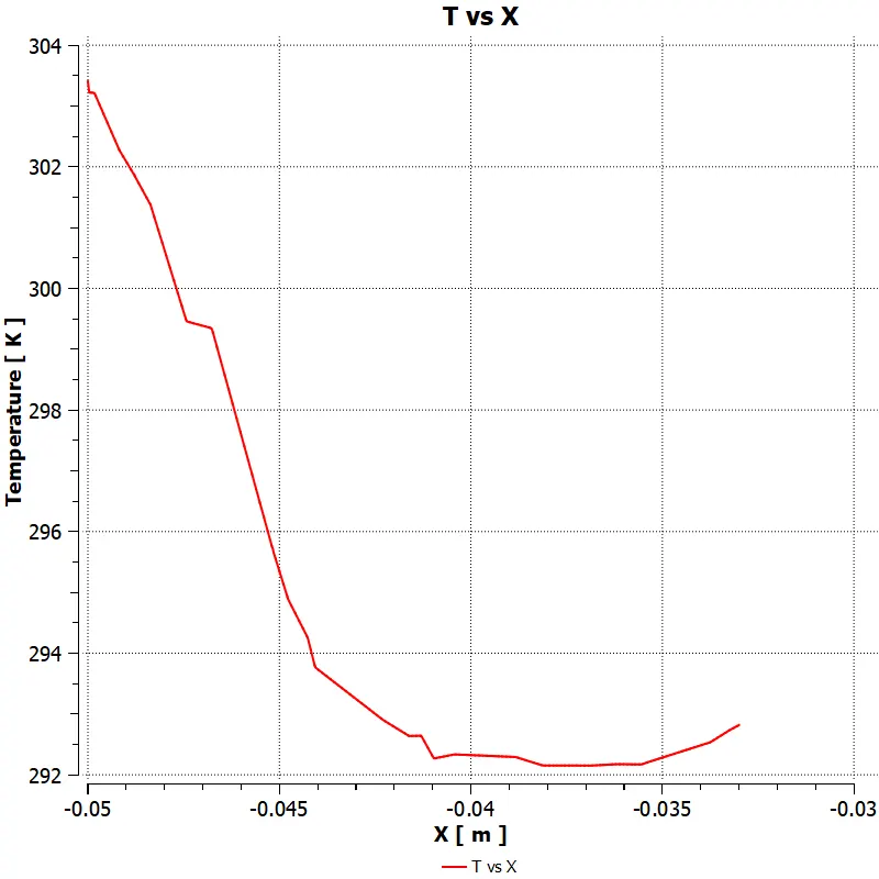
Temperature variation at the junction along X
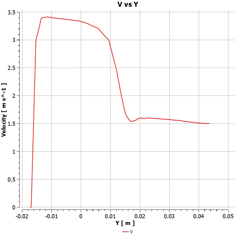
Velocity Variation along Y at Junction across the pipe or along cold inlet
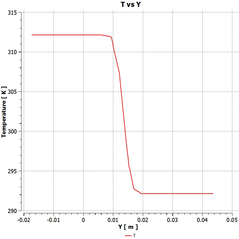
Temperature Variation along Y at Junction across the pipe or along cold inlet
Examining Results :
`h_(mix) = (m_(hot)*h_(hot) + m_(cold)*h_(cold))/(m_(hot) + m_(cold)`
`T_(mix) = (T_(hot)*h_(hot) + T_(cold)*T_(cold))/(m_(hot) + m_(cold)`
From Fluent we've :
Enthalpy
`h_(hot) = 10076.805`
`h_(cold) = 10076.805`
`h_(mix) = 10076.805`
Verifying with above equations
`h_(mix) = (10076.805*3 + 10076.805*1.5)/(1.5 + 3) = 10076.805`
Temperature
`T_(hot) = 39 C = 312 K`
`T_(cold) = 19 C = 292 K`
`T_(mix) = 35.01245 C = 308.01245 K`
Verifying with above equations
`T_(mix) = (312*3 + 292*1.5)/(3+1.5) = 305.333 K`
FOR CASE 2
Viscous effect - K epsilon model - Realize
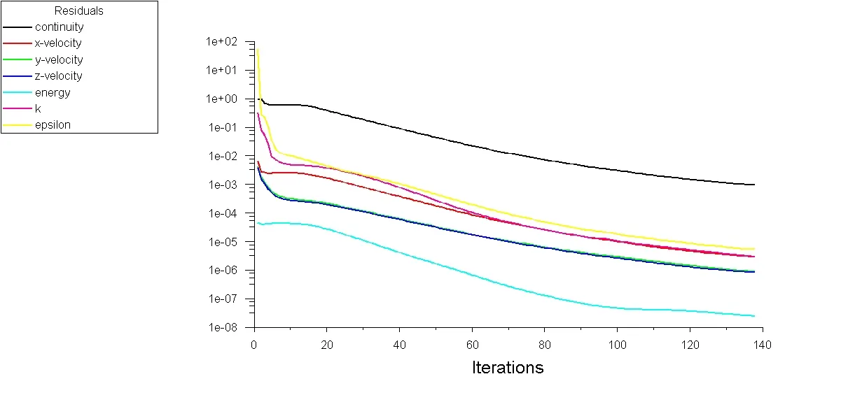
Convergence of Residual
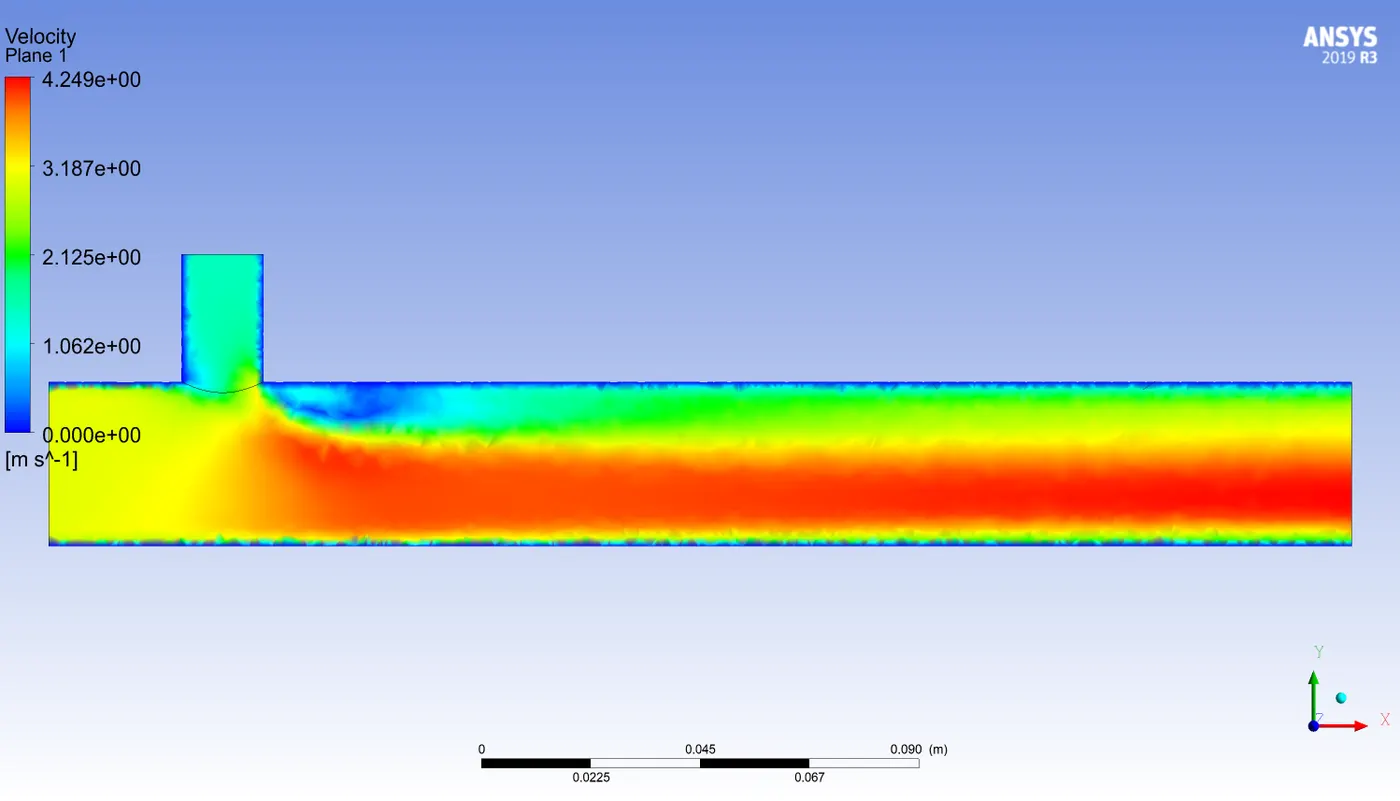
Resultant Velocity Variation on Plane
Temperature variation on plane
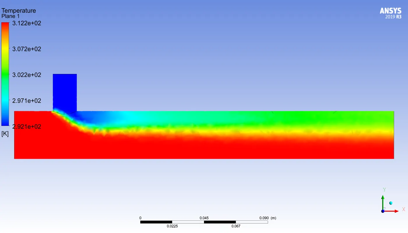
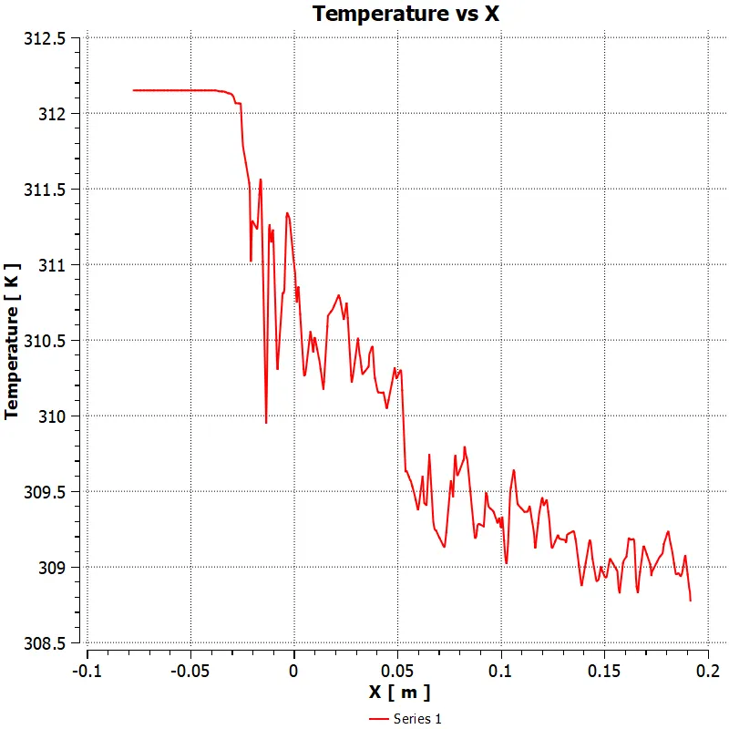
Temperature variation along the length
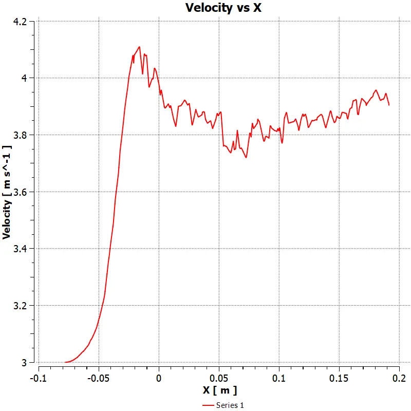
Velocity variation along X
Temperature and Velocity variation across the outlet
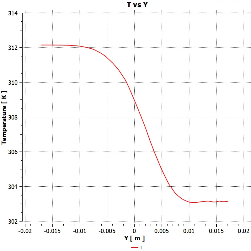
Temperature and velocity variation across the junction in the X direction :
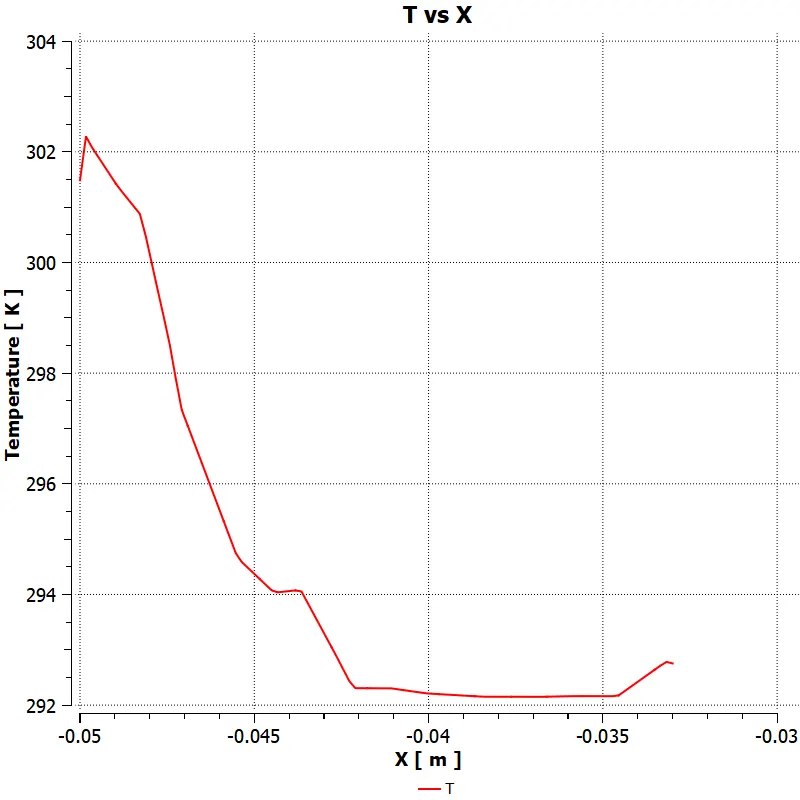
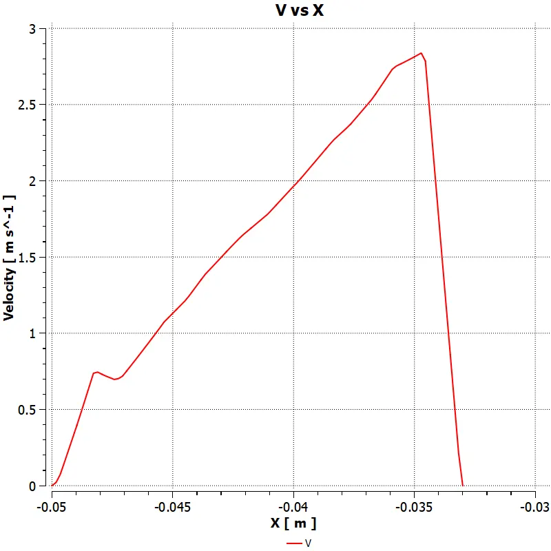
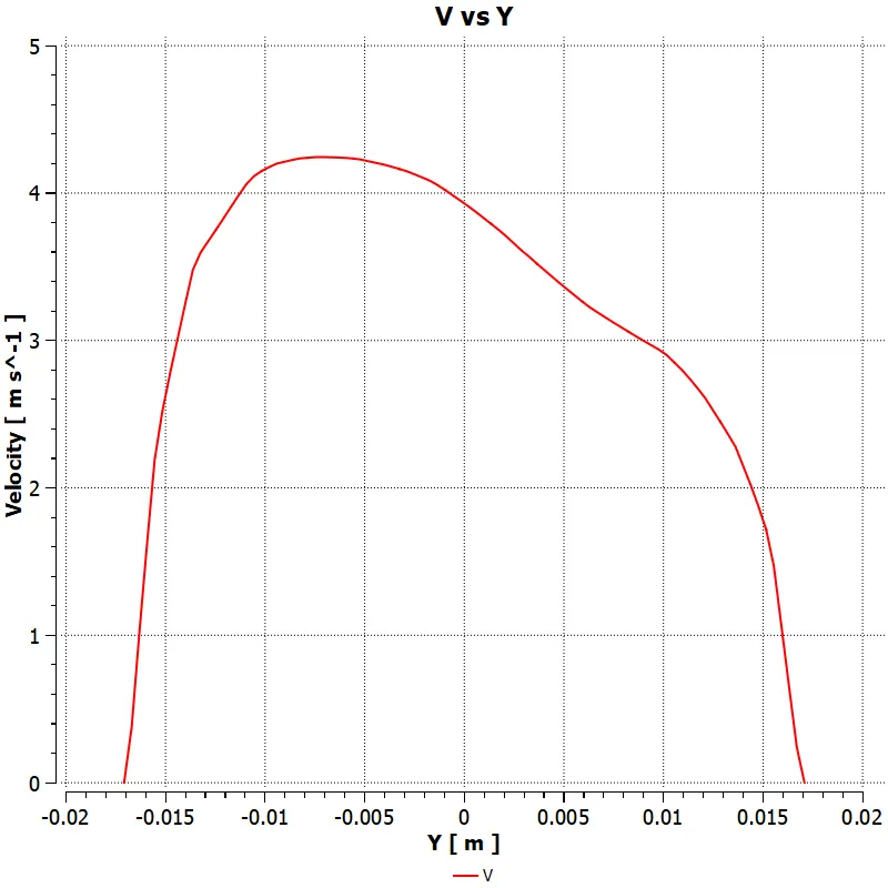
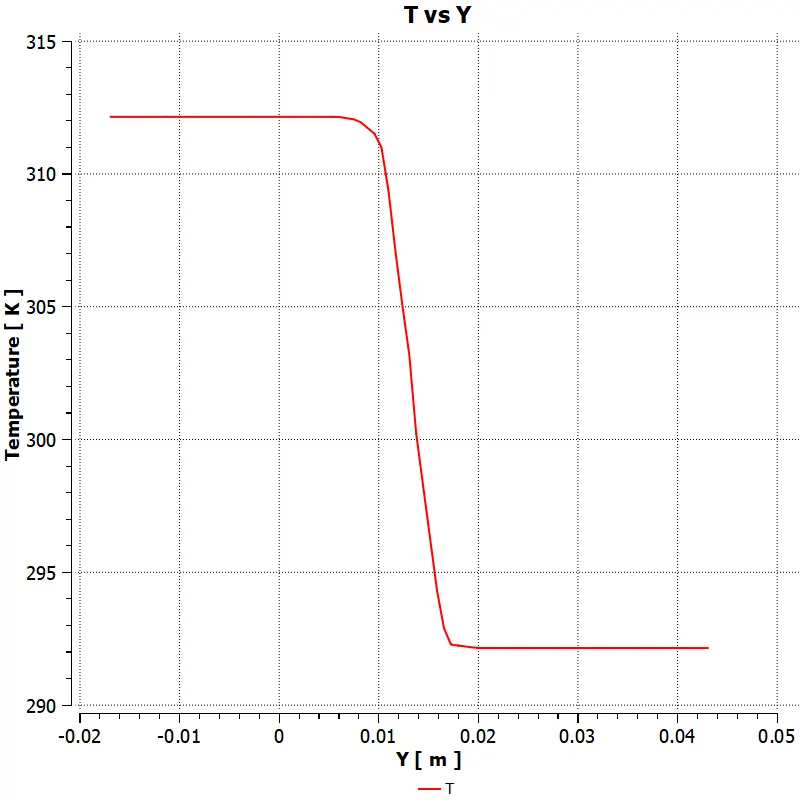
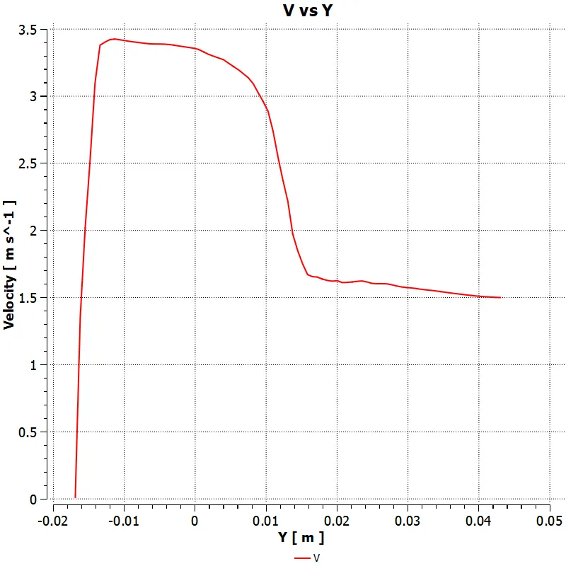
Velocity and Temperature variation at a junction along Y or along cold inlet
Examining Results :
`h_(mix) = (m_(hot)*h_(hot) + m_(cold)*h_(cold))/(m_(hot) + m_(cold)`
`T_(mix) = (T_(hot)*h_(hot) + T_(cold)*T_(cold))/(m_(hot) + m_(cold)`
From Fluent we've:
Enthalpy
`h_(hot) = 10076.805`
`h_(cold) = 10076.805`
`h_(mix) = 10076.805`
Verifying with above equations
`h_(mix) = (10076.805*3 + 10076.805*1.5)/(1.5 + 3) = 10076.805`
Temperature
`T_(hot) = 39 C = 312 K`
`T_(cold) = 19 C = 292 K`
`T_(mix) = 35.01245 C = 308.01245 K`
Mesh Independent Study for Case 1 :
Element Size = 0.002 m
Outlet T = 36.47 C
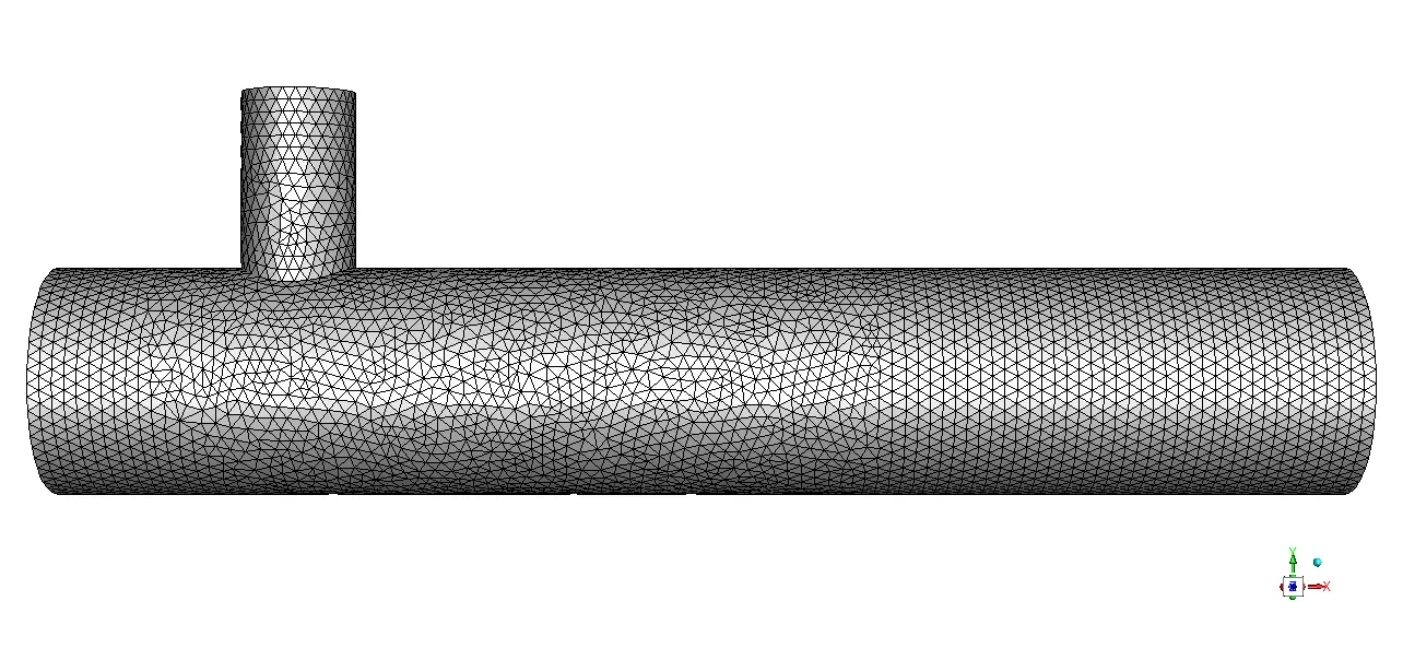
Element Size = 0.001 m
Outlet Temperature = 36.41 C
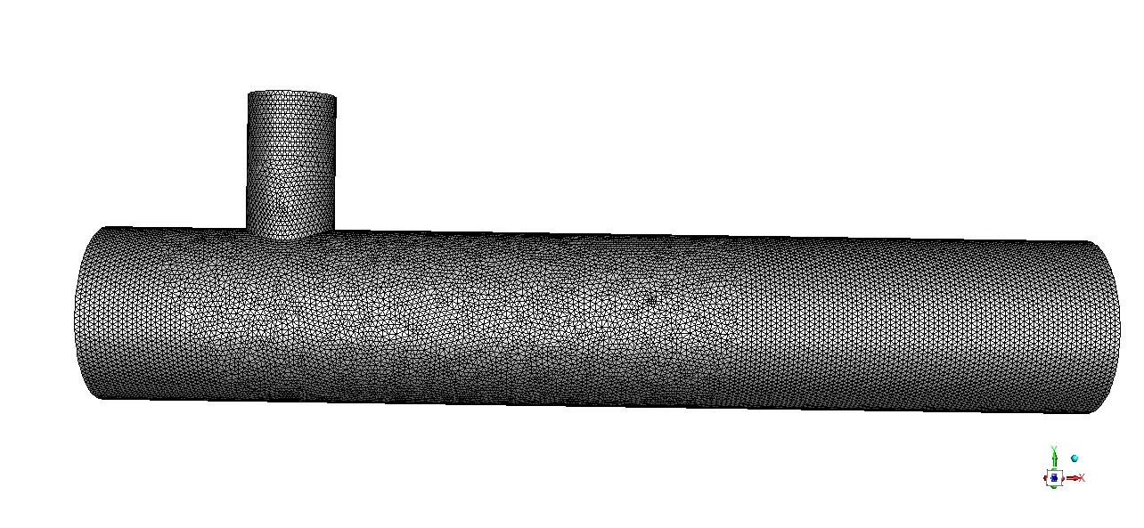
Element Size = 0.0009 m
Outlet Temperature = 36.42 C
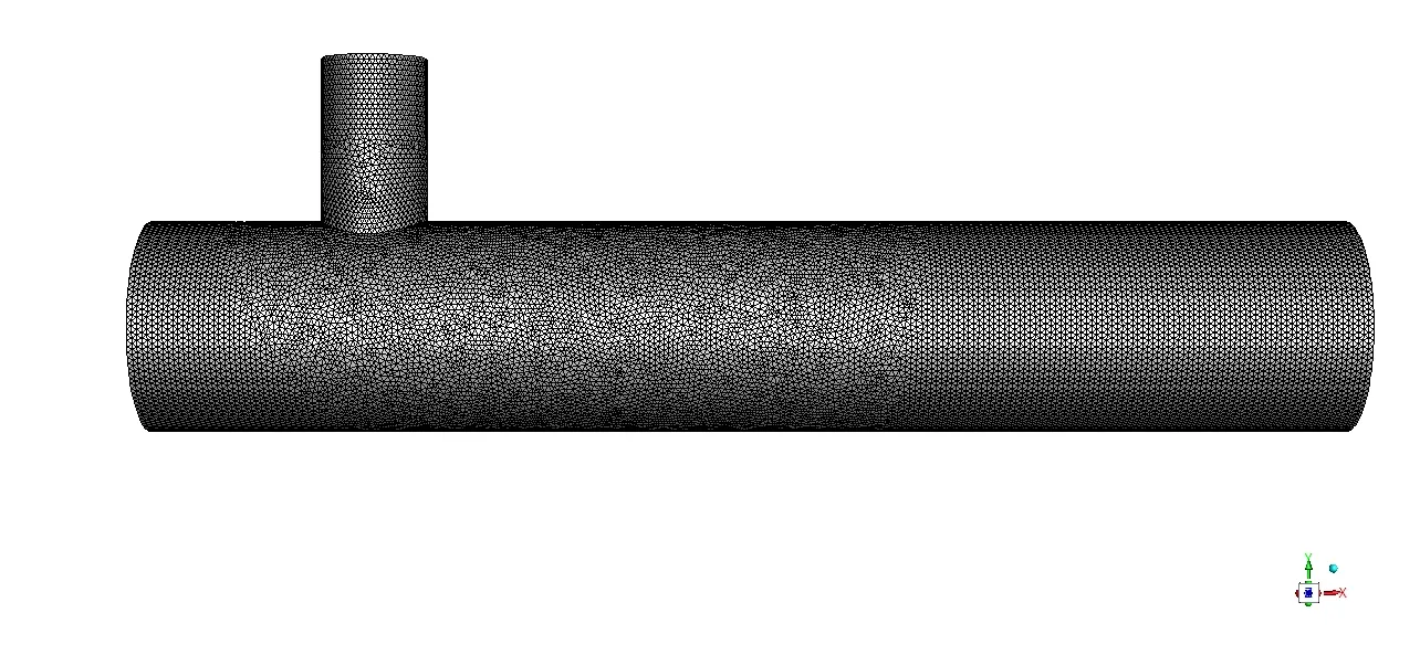
Element Size = 0.0008 m
Outlet Temperature = 36.42 C
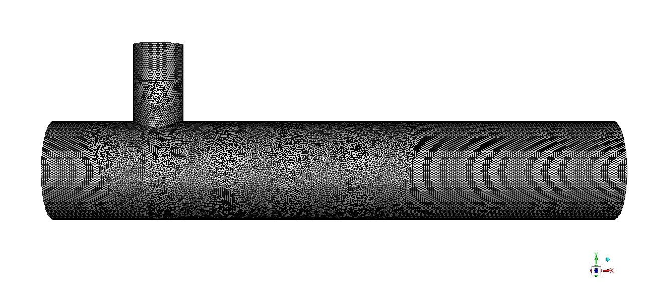
Element Size = 0.0007 m
Outlet Temperature = 36.42 C
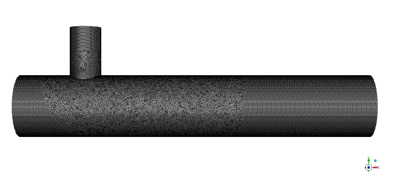
It can be observed that for element size less than 0.001 m our outlet temperature attains a stable value of 36.42 C
Conclusion
Effect of length
- If the length of the pipe is increased, by keeping all other factors like inlet temperatures, momentum ratio, etc.
- The Temperature at the outlet decreases.
- The standard Deviation is also less, that means the temperature on every point the outlet face is approximately equal to the average temperature of the face.
Effect of momentum Ratio
- If we increase the momentum ratio and keep all of the rest parameters constant.
- The temperature at the outlet decreases.
- If we decrease the momentum ratio and keep all of the rest parameters constant.
- Then the temperature at the outlet increases.