2D Element Formulation using RADIOSS

OBJECTIVE:

1. Import the Starter file.
2. Edit Run time and Anim DT.
3. Run the analysis and plot the Graphs.
4. In the second Case, change the recommended properties and run the analysis and plot for the same.
5. Compare the two cases and state the difference in the results.

PROCEDURE:

• CASE: 1 Import starter file
• Edit Run time and Tfreq
• Run the model
• Check the results
• Plot the graphs
• Explaining Recommended properties
• CASE: 2 Import starter file and change the properties
• Plot the graphs
• Compare CASE:1 and CASE: 2
• Hour galss and its method

CASE 1: IMPORT STARTER FILE

Go to Files in task bar >> Import >> Solver Deck >> FIRST_RUN_0000.rad (select) >> Import

The starter file stores information about:

• Nodes
• Load Conditions
• Velocity
• Boundary Conditions, etc.
• Basically, it is an ASCII(American Standard Code for Information Interchange) file that contains the model information.
• The starter file should always end with 0000.rad.

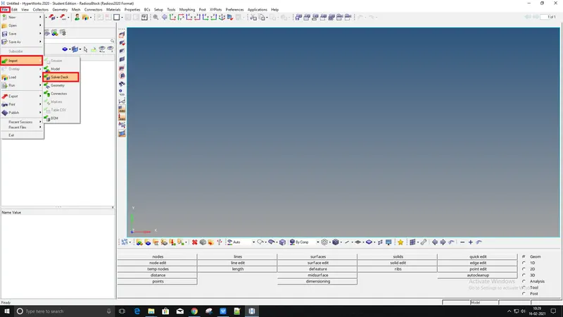
IMPORTING SOLVER DECK FILE

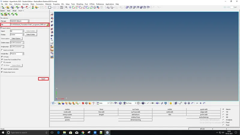
SELECTED STARTER FILE FROM THE FOLDER

CLICK IMPORT

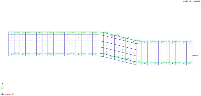
MODEL IMPORTED

1. Using the crash beam file from the previous assignment, change the run time to 55 ms.

EDIT RUN TIME AND Tfreq:

To change Tstop and Tfreq

Go to Model browser >> Select Cards >> ENG_RUN >> Then below one task editer will open their Update Tstop as 55

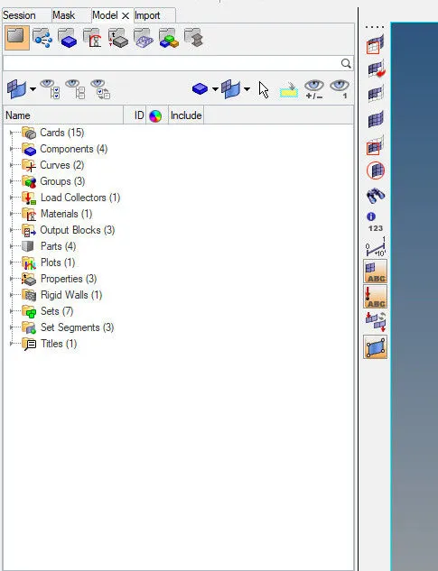
SELECTED MODEL BROWSER

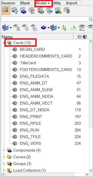
CARD

Run time (Tstop):

The Run time is the total time taken for the the sound wave to travel through the entire length of the model.

This should be calculated by a formula i.e, Total length/Speed of sound

Here we don't have to calculate Tstop because its already given as 55

So, here we just have to edit the Tstop time

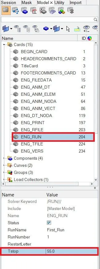
EDITED Tstop

2. Change the number of animation steps during simulation to a minimum of 25 and maximum of 60.

Tfreq:

Change the Number of Animation steps

This should be calculated by a formula i.e, Run Time/Number of animation steps

Animation frequency= 55/30 = 1.8333

Go to Model browser >> Select Cards >> ENG_RUN >> Then below one task editer will open their Update Tfreq as 1.8333

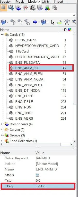
EDITED Tfreq

3. Run the base simulation without any modification to element properties.

RUN THE MODEL:

Now we have to run the analysis from the Analysis module:

Analysis >> Radioss >> Input File: Starter file ) >> Radioss

The input file is the same Started file that we had just Edited.

Once we hit Radioss, a pop-up box will appear. It shows us the real time analysis and gives us the final result.

After run the file will contain animation video along with animation steps and time history file will be saved in the same folder where the starter file exists.

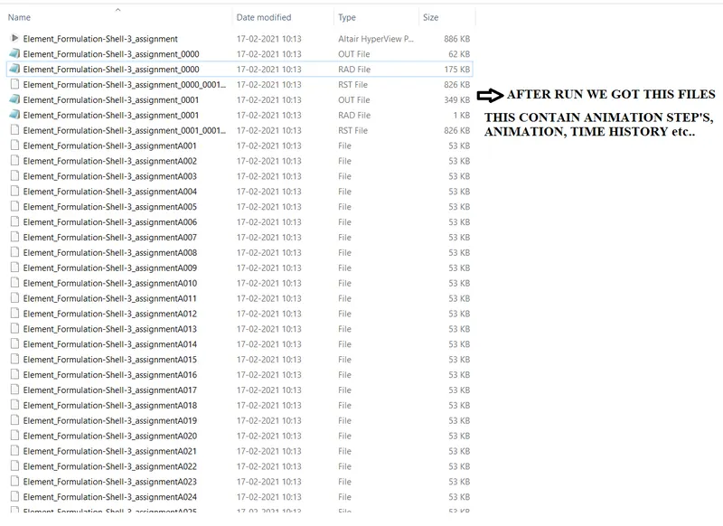
4. At the end of the simulation, do the energy error and mass error checks and determine whether results would be acceptable.

CHECK THE RESULTS:

A Engine Output file of 001.out format is generated after analysis.

The Engine Output file contains the data during simulation, such as:

• Cycle Time Step
• Energy Error
• Mass error
• Internal Energy
• Kinetic energy
• Contact energy

Here we have to check for the energy and Mass error.

1. It is normal if the error slightly increases .
2. The energy error acceptable in the Range of -15% to +5%.
3. The mass error acceptable in the Range of 0 to 2.

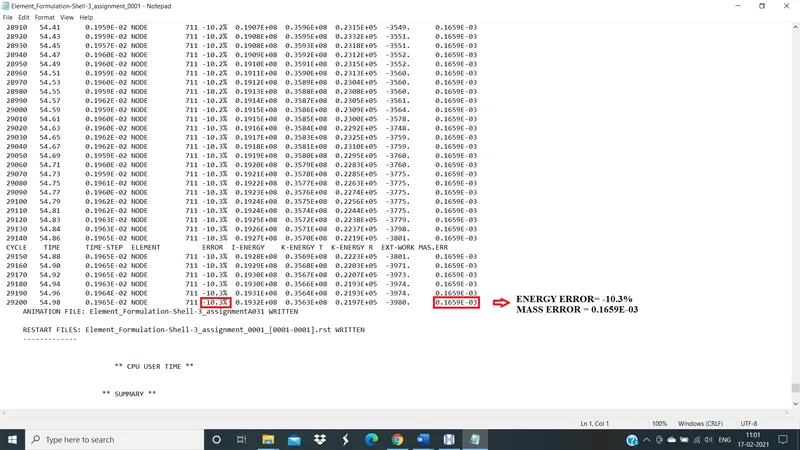
Here we have Energy error as -10.3% and Mass error as 0.1659 E-03.

This two are in the acceptable range

But here energy error is increasing because of Hourgalss

Here the Negative sign indicates that there is an energy dissipated from the system or loss of energy

PLOTS THE GRAPHS:

Review the Simulation

We have to import the animation file in HyperView first:

HyperView >> Select File >> FIRST_RUN. h3d >> Apply

• HyperView is a post processing and visualization environment for FEA that gives the output of the analysis in a simulations format that is How the impact force affects the model.
• The different regions of deformations.
• Where the bending starts.
• Where the Max stress present
• Where the hourgalss forming etc..

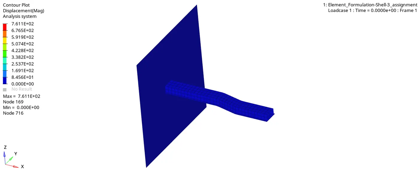
CASE:1 HYPERVIEW ANIMATION

Here we can clearly see that where exactly the maximum and minimum displacement happen

Now plot the graphs

Hypergraph 2D >> Data File >> FIRST_RUNT01 >> Apply

Hypergraph is a data analysis and plotting tool that represents the FEA from the simulation in graphs with respect to the selected unit system.

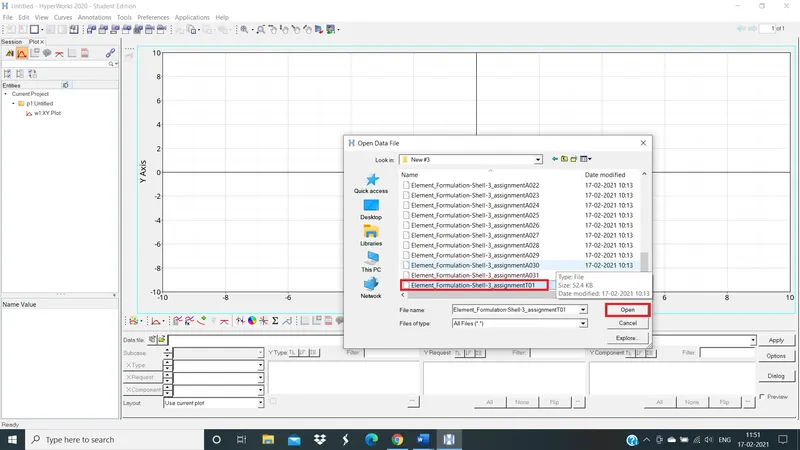
SELECTING TIME HISTORY FILE

Plot graphs for rigid wall forces of the simulations

SELECTING RIGIT WALL FORCE

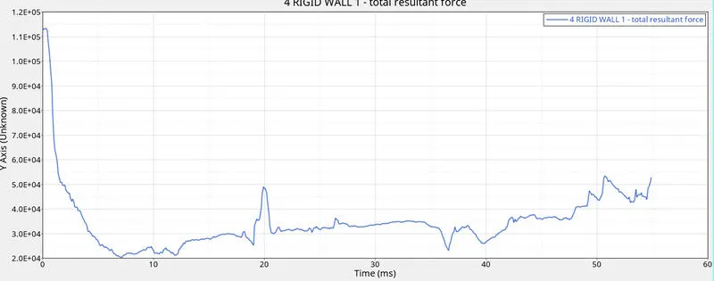
GRAPH PLOTTED FOR RIGID WALL FORCES

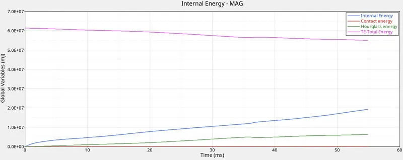
Plot graph for internal energy, hourglass energy, contact energy, total energy

SELECTING GLOBAL VARIABLES

GRAPH PLOTTED FOR GLOBAL VARIABLES

CASE 2:

RECOMMENDED PROPERTIES:

Parameters		Comment
Ishell =24		QEPH 4 nodes shells are best combination of cost and accuracy.
Ismstr=2		Full geometric nonlinearities (default)with possible small strain formulation activation in RADIOSS Engine.
Ish3n=2		Standard 3 noded shell (C0)with modification for large rotation(default)
N=5		Number of integration points set to 5 for accuracy bending.
Ithick=1		Thickness change is taken into account for accuracy.
Iplas=1		Iterative plasticity for good accuracy.

Changing the properties with given shell properties

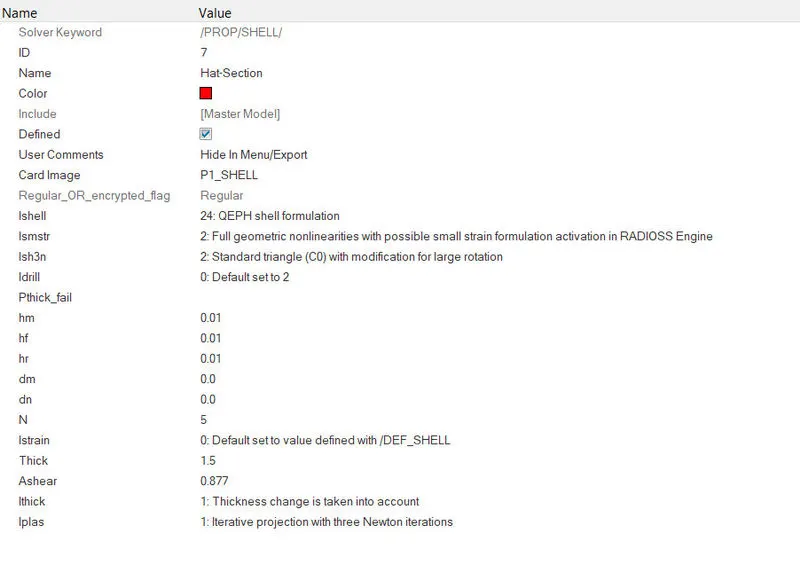
WITH RECOMMENDED PROPERTIES

Save as new file in new folder then change properties

Now RUN the Radioss

as shown in above steps

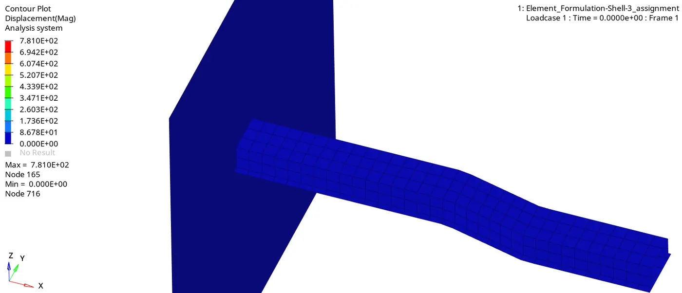
CASE: 2 HYPER VIEW ANIMATION

Here we can clearly see that where exactly the maximum and minimum displacement happen

Now plot the graphs

Hypergraph 2D >> Data File >> FIRST_RUNT01 >> Apply

Hypergraph is a data analysis and plotting tool that represents the FEA from the simulation in graphs with respect to the selected unit system.

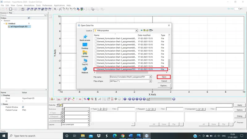
TIME HISTORY FILE

Plot graphs for rigid wall forces of the simulations

SELECTED RIGID WALL

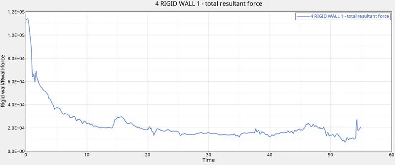
GRAPH PLOTTED FOR RIGID WALL FORCES

Plot graph for internal energy, hourglass energy, contact energy, total energy

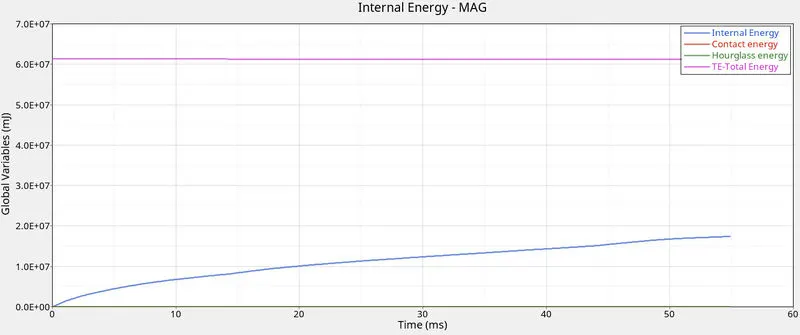
GRAPH PLOTTED FOR GLOBAL VARIABLES

COMPARING RESULTS:

CASE:1 CASE:2

Max value = 113439.45 Max value = 114153.79

Min value = 20376.56 Min value = 7655.16

RIGID WALL FORCES COMPARISON:

In case 1: The Component or rail is in contact with the wall so the Force acting on that area is at peak. As the simulation starts the contact decreases and so force and at the end of the simulation the area of the crushed component is again in contact with the wall hence the rise of force at the end of graph.

In case 2: The Component or rail is in contact with the wall so the Force acting on that area is at peak. but when the simulation starts the area of contact decreases gradually and varies hence the force acting varies throughout and decreases at end.

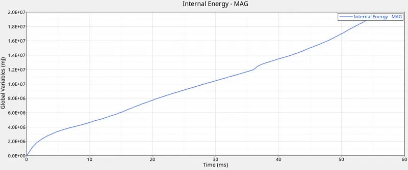
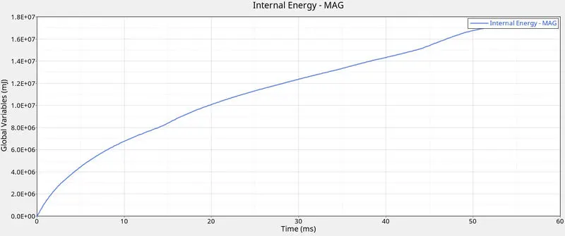
Max value = 19285676 Max value = 17465234

Min value = 0 Min value = 0

INTERNAL ENERGY COMPARISON:

The Case 1 has undergone more deformations resulting in higher Internal energy. The Internal energy is the Strain energy that is absorbed by the element.

In case 2 comparetivly less

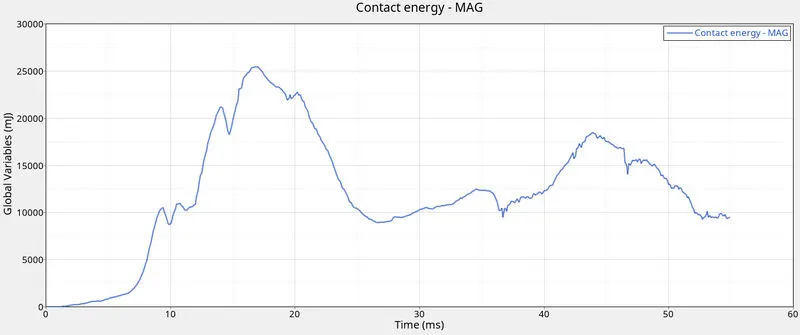
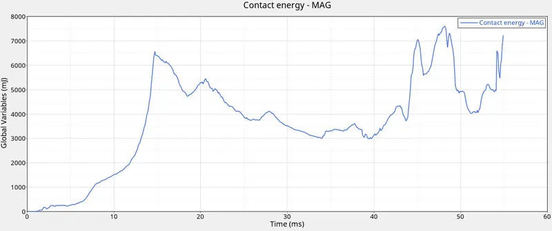
Max value = 25441.50 Max value = 7598.85

Min value = 0 Min value = 0

CONTACT ENERGY COMPARISON:

Due to the increase in stiffness, the elements in case 2 offers better resistance to the external force. Therefore, the max contact force in case 2 occurs towards the end of the run time.

where as in case 1, it happens in the beginning.

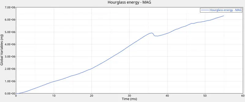
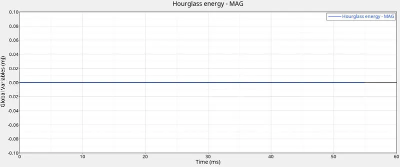
Max value = 6315967.50 Max value = 0

Min value = 0 Min value = 0

HOURGLASS ENERGY COMPARISON:

In case 1 its increases with respect to time

So, when I shell =0 it takes the default information which is I shell =1 and that is Q4 under integrated element with single integration point.

Where as in case 2 Stays zero with respect to time.

I shell =24 having under integrated element with single integration point though uses Physical stiffness method which avoids hour glass before even it is generated.

case 1 uses Q4 elements which are more prone to Hourglass effect. Hence, there is an increment in the Hourglass energy. Where as in case 2, there is no hourglass effect due to QPEH elements

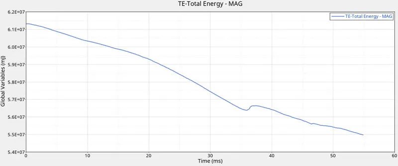
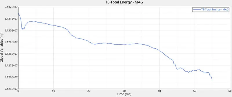
Max value = 61314900 Max value = 61314900

Min value = 54965860 Min value = 61257480

TOTAL ENERGY COMPARISON:

It is the sum of Internal energy, Kinetic energy, and external work.

In case 2 we can say a hike during Bending which indicates that the strain energy is increased while bending indicates that the elements are offering better resistance to bending. But the curve is almost linear in case 2, there is a small hike at Buckling region alone indicating the resistance to Buckling and increase in Total energy.

In case 1 due to some energy dissipation there is a slight decrease in total energy towards the end Hence the graph curve decreases.

HOURGLASS AND ITS CONTROL METHODS:

Hourglass is a situation where node is moving but nothing is being recorded.

So, Stress won't develop on the rest of the nodes.

Therefore, Timestep cycle is broken as there is no dissipation of force to the next node and so on.

There are 2 methods to control the Hourglass effect:

Sl. No.	Perturbation Method	Stabilization Method
1.	High Velocity/strain rate problems	Low velocity/strain rate problems.
2.	Bad behaviour in: i. Large deformations ii. elastic loading-unloading cycles	Accurate in Loading and Unloading cycles, even if there is hourglass.
3.	Inhibits Hourglass deformation.	Reduces the existing Hourglass deformation.
4.	Can't recover.	Recovery is possible.
5.	Hourglass coefficient remains same or increases.	Reduces hourglass coefficient.
6.	On Q4 elements.	On QPEH elements.

CONCLUSION:

I would like to conclude that this assignment helped me to understand how to change the run time, Anim DT and how to change the material and how to plot the required graphs and how to study them.