AIR STANDRAD CYCLE - Otto Cycle using Matlab

AIM : To create a program using MATLAB for plotting Pressure vs Volume diagram for an well known Air Standard Cycle i.e. Otto Cycle and to find its Thermal Efficiency(Ƞ) of the engine.

THEORY :

• The modern petrol (gasoline) engines operate on otto (constant volume) cycle. This cycle was introduced by a German scientist Nicolaus otto in 1876.
• This cycle describes about the changes to a mass of gas as it is subjected to changes of pressure, temperature, volume, addition of heat, and removal of heat.
• The ideal Otto cycle consists of two constant volume and two reversible adiabatic or isentropic processes shown on PV diagrams.

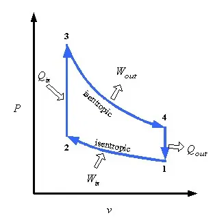
• Process 1–2 is an isentropic (adiabatic) compression of the charge as the piston moves from bottom dead centre (BDC) to top dead centre (TDC).
• Process 2–3 is a constant-volume heat transfer to the working gas from an external source while the piston is at top dead centre.
• Process 3–4 is an isentropic (adiabatic) expansion (power stroke).
• Process 4–1 completes the cycle by a constant-volume process in which heat is rejected from the air while the piston is at bottom dead centre.

GOVERNING EQUATIONS :

1. Equation to Trace volume in otto cycle -

`V/Vc=1+1/2 (cr-1) [ R+1-cosθ-(R^2-sin^2 θ)^(1/2) ]`

2. Equation to calculate Thermal Efficiency in an Otto Cycle –

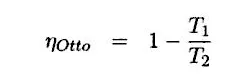
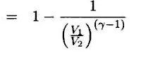
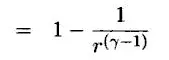
where, r = cr(compression ratio) =`V_s / V_c`= `V_1/V_2`

OBJECTIVES OF THE PROJECT:

• To plot the PV Diagram for Otto cycle (Air Std Cycle) by creating a code using MATLAB.
• To find the Thermal Efficiency of an engine for Otto cycle.

• FUNCTION CODE -

function [V] = Engine_kinematics(Bore,Stroke,Connect_rod,cr,start_crank,end_crank)

a = Stroke/2;
R = Connect_rod/a;

v_s = pi/4*Bore^2*Stroke;
v_c = v_s/(cr-1);

theta = linspace(start_crank,end_crank,100);

term1 = 0.5*(cr-1);
term2 = R+1-cosd(theta);
term3 = (R^2-sind(theta).^2).^0.5;

V = (1 + term1*(term2-term3)).*v_c;

end

• MAIN CODE -

%% Code for Otto Cycle
clear all
close all
clc

% Inputs -
gamma = 1.4;
t3 = 2300;

% State variables -
p1 = 101325;
t1 = 500 ;

% Engine Geometric Parameters -
Bore = 0.1;
Stroke = 0.1;
Connect_Rod = 0.15;
cr = 12;

% Calculating the swept volume and clearance volume -
v_swept = (pi/4)*Bore^2*Stroke 
v_clearance = v_swept/(cr-1)
v1 = v_swept + v_clearance
v2 = v_clearance

% State variables at pt.2 -
%(p2v2)^gamma = (p1v1)^gamma
% p2 = p1*(cr)^gamma
p2 = p1*(cr)^gamma

% p1v1/t1 = p2v2/t2
t2 = p2*v2*t1/(p1*v1);

constant_c = p1*v1^gamma;
V_compression = Engine_kinematics(Bore,Stroke,Connect_Rod,cr,180,0);

P_compression = constant_c./V_compression.^gamma;

% State variable at pt.3 -
v3=v2 % As it is a Constant volume process

%p3v3/t3=p2v2/t2
%p3=p2*t3/t2
p3 = p2*t3/t2 

constant_c = p3*v3^gamma;
V_expansion = Engine_kinematics(Bore,Stroke,Connect_Rod,cr,0,180);

P_expansion = constant_c./V_expansion.^gamma;

% State variables at pt.4-
v4 = v1 

% (p3v3)^gamma = (p4v4)^gamma
% p4 = p3*(v3/v4)^gamma
p4 = p3*(v3/v4)^gamma

% Plot 
figure (1)
hold on
plot(v1,p1,'*','markersize',5,'color','r')
plot(V_compression,P_compression,'linewidth',1)
plot(v2,p2,'*','markersize',5,'color','r')
plot(v3,p3,'*','markersize',5,'color','r')
plot(V_expansion,P_expansion,'linewidth',1)
plot(v4,p4,'*','markersize',5,'color','r')

plot([v2 v2],[p2 p3],'color','b','linewidth',1)
plot([v1 v4],[p1 p4],'color','b','linewidth',1)
xlabel('Volume(V)')
ylabel('Pressure(P)')
title('Pressure Vs Volume Diagram for OTTO CYCLE')

% Thermal efficiency for an Otto Cycle-
n = (1-(1/cr^(gamma-1)))*100;
Thermal_efficiency = n

• OUTPUTS FOR THE CODE –

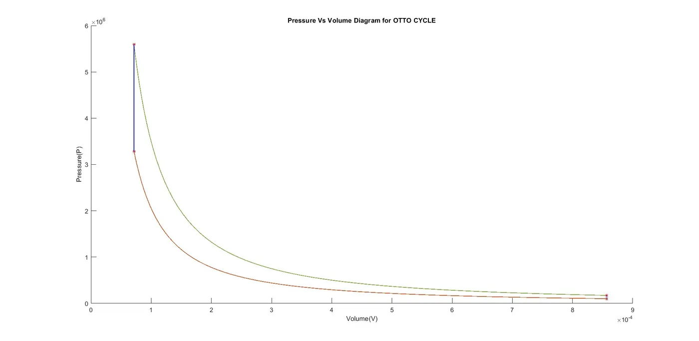
The above plot shows the pressure vs volume graph for otto cycle in which volume decreases from state 1-2 during compression and increases from state 3-4 during expansion process.

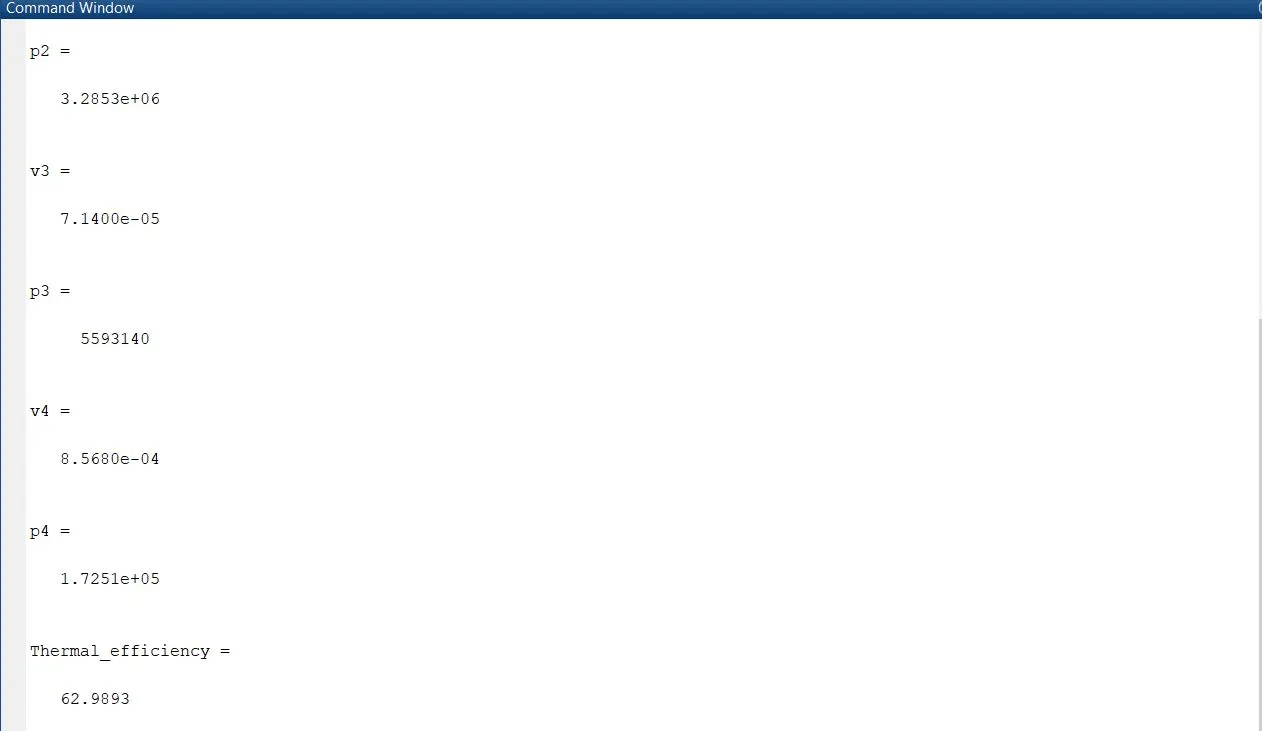
The above image shows the thermal efficiency for an otto cycle after calculating all the state variables for pressure and volume.

STEPWISE EXPLANATION OF THE CODE –

1. In this program inputs like gamma, t3 and state variables like p1, t1 are assumed matching the requirement of otto cycle and also the engine geometric parameters are taken into consideration.
2. In the main code for Otto cycle we are calculating the swept volume(Vs) and the clearance volume(Vc) and then v1 and v2.
3. Also, initially we are defining a function for piston kinematics in new script that will be the function code for otto cycle.
4. In the function code we have used a equation to trace volume for an otto cycle and giving the values for theta from the start of crank to end of crank rotation by using command linspace.
5. We had save the Function code for file name Engine_kinematics and used the same name in defining and calling the function.
6. Then, we had called the function in the main code in otto cycle to trace the volume and pressure from pt.1-2 and 3-4 respectively.
7. Then calculated the other state variables at pt. 2,3 & 4 respectively.
8. Finally, plotted the PV diagram using plot command in MATLAB and calculated the thermal efficiency for an otto cycle using its equation respectively.

Errors faced while programming –

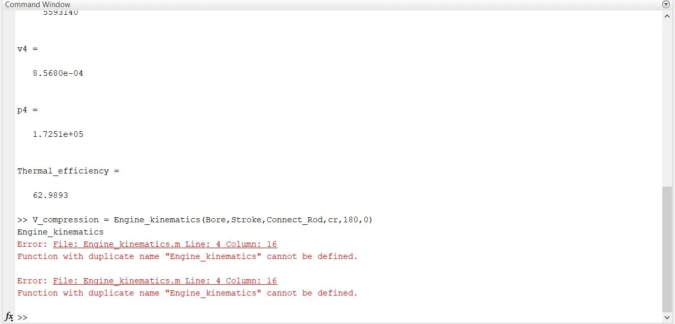
• Error for calling the function - Function with duplicate name "Engine_kinematics" cannot be defined.

Reason – Initial start of code with Use of clear all ; close all ; clc ; command in the function code.

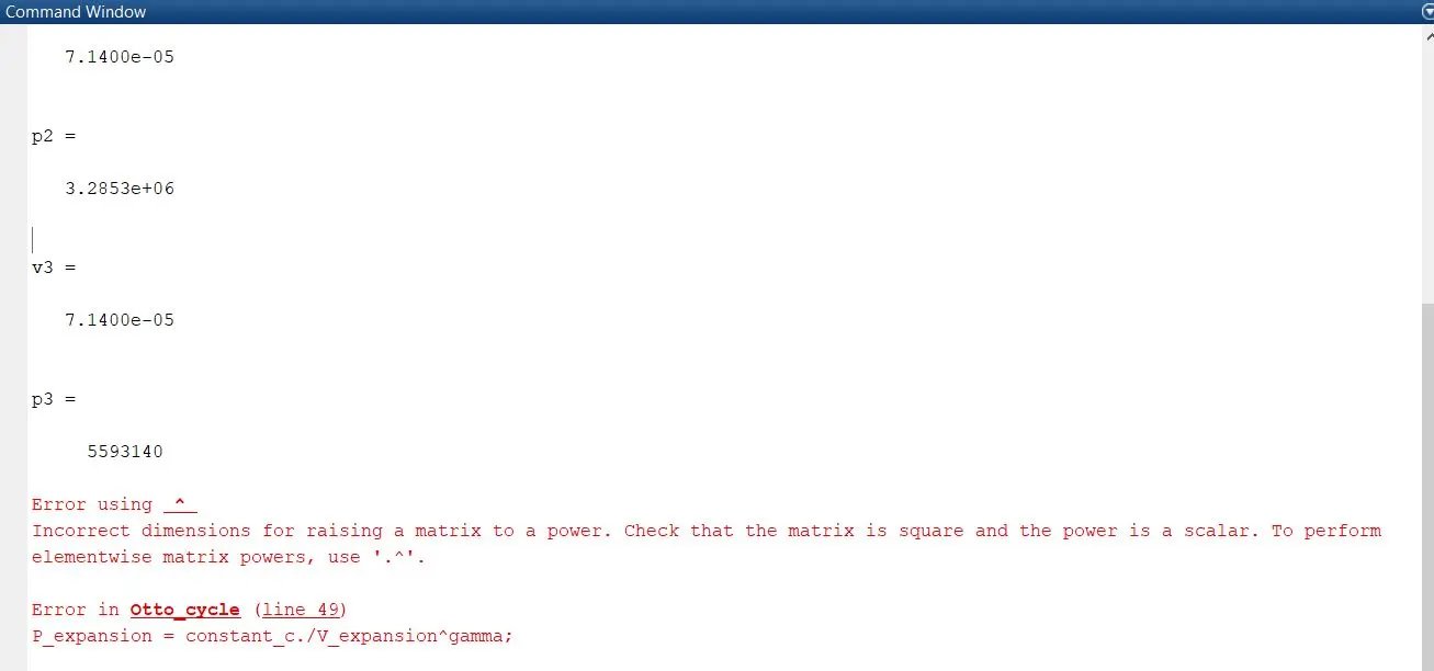
• Error in P_expansion line in Main code - Incorrect dimensions for raising a matrix to a power.

Reason – Use normal of power expression to raise a power of matrix ^ instead of elementwise matrix power.

Steps taken to overcome the Errors Faced –

1. Eliminated the use of clear all ; close all ; clc ; command in the function code at start of it to fix the Error in function code.
2. Use the elementwise matrix power .^ for raising a matrix to a power -V_expansion.^gamma had fixed the issue.

Screenshots showing errors thrown in command window –

Error for calling the function

Error in P_expansion line in Main code

CONCLUSION –

Thus, we get an brief idea about creating a program using piston kinematics for plotting PV diagram for an otto cycle where volume changes isentropically from process 1-2 and 3-4 respectively. Also, we had calculated thermal efficiency of an engine for an Otto cycle which is 62.98 %.