Differences Between Skew and Frame

Any CAE or CAD software has its own coordinate system. It is the first visible entity in the software’s GUI and is called the global coordinate system. All the parts attached to a model will follow this coordinate system if it is moved or translated likewise. 

Let’s take a scenario where a particular part is tilted at an angle or the force/displacement only acts on a particular local region. At those times, one cannot rely on a global coordinate system. This issue can be avoided if any coordinate system is available exclusively for that part alone. This exclusive coordinate system for just only a part is called the local coordinate system. If a local coordinate system is established, the model will move only on that particular defined coordinate system and not follow the global coordinate system. 

Likewise, RADIOSS provides local coordinate system options as well. Still, there are some very minute differences in them and also, one cannot outrightly say they don’t follow the global coordinates.

Skews

• Skew is a type of reference coordinate system that helps define local quantities concerning the global coordinate system.
• It remains in a fixed position even if it is a fixed skew or moving skew.
• In a moving skew, the orientation of the node of interest is recomputed every time, with that of the origin coordinates of the skew. 
• Skew is the most widely used in most of the RADIOSS inputs.
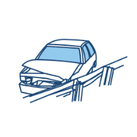
• An example is the study of intrusions in the car through skews. 2 nodes are created, and fixed skews are assigned to them. The travel of the node is computed from the global coordinates, and it is presented in the local coordinates. The overall travel of the node is obtained.

 

 

Frames

• The frame is a type of reference coordinate system where the quantities defined follow their own origin.
• Here, unlike the moving skew, the moving frame is attached to the node, which is selected as the origin.
• It calculates the motion of the body relative to the frame defined.
• Frames are used only for options like imposed velocity, imposed displacement, TH/node etc.,

 

 

Difference between Moving Skew and Frame

• To understand moving skew and moving frame better, let’s look at figure 3.
• Let’s consider two nodes N1 and N2 are moving in the direction mentioned. The node N1 is the origin of a moving skew, and N2 is our node of interest. N1` and N2` is the new position of the N1 and N2 nodes. 
• Here as seen before, what moving skew does is, at the first step, the skew will be present as usual in its origin node position. In the next step, the moment the nodes move, the skew that is created with respect to the position of node N1 will remain fixed at the same position of the N1 node coordinate. 
• With respect to this position, the displacement of node N2 is calculated. In a nutshell, even if a moving skew is created, the skew is fixed at the position of the origin node selected.

 

 

• In Frame, the situation is opposite. The frame is attached to the origin node if a moving frame is selected, as mentioned above. If the origin node moves from its position N1 to N1`, the frame also moves from N1 to N1` i.e it gets attached with the selected origin node and moves along with it.

 

 

All four options are available for creating a local coordinate system, but at the end of the day, it depends on what RADIOSS requires. If a particular option like accelerometer, initial velocity etc, requires ISKEW input, then only skew can be defined. If a frame is selected instead of skew, it throws an error in the status bar. So the selection of Skew or Frame is based on the use case in those options.

 

1) Representation of the Skews and Frames

 

• The image below is an example of a fixed skew/frame and its representation in the .rad file.
• The OX, OY, OZ coordinates are the origin points, X1, Y1 and Z1 is the point that displays the direction of the axis. If X1 is denoted as 1 then the axis selected in the panel is X axis. The same applies for Y1 and Z1 as well.
• The coordinates X2, Y2 and Z2 are the point displays which plane is selected, if the plane is selected as the XY plane from the option, then X2, Y2 is displayed as 0 and Z2 is displayed as 1 as shown below in the image.

 

 

• The image below is an example of a moving skew/frame and its representation in the .rad file.
• Only three values are present; those are nothing but the N1, N2 and N3 node IDs. Here, N1 displays the origin node, N2 is the axis node, and N3 is the plane node.

 

 

 

2) Differences in creating a fixed skew/frame and moving skew/frame

 

• While creating a fixed skew/frame or moving skew/frame, there is a slight variation in the creation of fixed and moving skew/frame.
• When a fixed skew/frame is selected, the ‘create by axis direction’ is displayed, and when the moving skew/frame is selected, the ‘create by node reference’ option is displayed.
• This difference is that the ‘create by axis direction’ option provides more flexibility with the selection of any kind of axis, namely x, y, z and their associated planes as shown below in the image

 

 

 

• The create by node reference option is displayed for moving skew/frame where the user can just select between the X and Z axis only. The plane selection also lies between xy or yz planes only.

 

 

Now let’s see a classic example of a Moving Skew. 

• Let's take the roof crash analysis; the roof needs to be moved by entering the imposed displacement in the model. In the roof, a moving skew is created on the master node of the rigid body.
• From the image shown below, the X axis is showing in the upward direction.

 

 

• The impactor must be moved in the X direction, towards the car, but there is another boundary condition where the rigid body is fixed in all the directions except the X shown below in the image,

 

 

• Now, if the boundary condition is applied to any other direction other than X, then it will throw an ‘incompatible kinematic condition’ error as shown below.

 

 

• From this, it can be concluded that whatever boundary conditions one is going to apply, when the skew is defined, the direction of boundary condition should be with respect to the skew and not based on the global. This is because, there may be some other boundary condition applied like the above mentioned, which might be contradicting and lead us to incompatible kinematic condition. Once this is fixed, like changing the direction of motion to X, the simulation goes through smoothly without any errors as shown below