Week 9- Unsteady moving zones Approach
Aim
To simulate the motion of the blades in a generic turbomachinery component using an unsteady approach running at 300 rpm.
Introduction
The unsteady approach uses a moving mesh method where the motion of the mesh is conducted across timesteps to simulate the system. In this approach, it is important to determine a suitable timestep size to ensure the proper simulation of the system. This can be done by checking the CFL number and making sure it is equal to or less than 1.
CFL- Courant–Friedrichs–Lewy Number:
The CFL number expresses the distance each piece of information passes through within a single time step. A CFL = 1, implies that the information is passing through one cell between each time step. A CFL >1 implies the information is skipping a few cells, and a CFL<1 implies the information will need additional time steps to leave the cell. Higher CFL numbers provide faster and less accurate solutions which are also prone to divergence. Lower CFL numbers provide much slower simulations with higher stability and accuracy. A CFL close to 1 or 0.7 is ideally the best suited for most applications. The CFL number is estimated by the following equation:
`CFL = u * (Delta t)/ (Delta x)`
where,
u - velocity magnitude of the flow [m/s]
`Delta t ` - time step size [s]
`Delta x` - length between mesh elements [m]
Method
Domain and Mesh
The meshed domain was provided and can be seen in the image below.
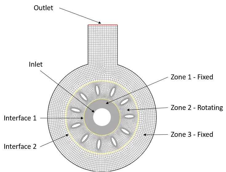
The domain consists of three fluid zones each separated by an interface marked in yellow. Zone 1 is stationary and consists of the inlet where the fluid will enter the domain. Zone 2 is rotational and consists of the airfoil setup. Zone 3 is stationary and consists of the outlet where the fluid will leave the domain. Interface 1 and interface 2 will act as the medium for fluid to pass through between the respective cell zones.
CFD Setup
The simulation was conducted on ANSYS Fluent 2022R2. Air was used as the fluid with default properties. Zone 2 was set to a rotational mesh motion with an rpm of 300. The airfoils in the zone were set as moving walls with rotational motions set relative to the adjacent cell zone. The inlet and outlet were set to a pressure inlet/outlet respectively with 0 gauge pressure.
The unsteady pressure-based PV-coupled solver was used to discretize the flow parameters. Turbulence in the flow was predicted using the two-equation Realizable K-Epsilon model with enhanced wall treatment. The second-order scheme was used to estimate the pressure, the second-order upwind scheme was used to estimate momentum and turbulence parameters. The solution was initialized by a standard initialization. Convergence was checked by scaled residuals achieving 1e-3 units and change in mass-flow rate at outlet not exceeding 1e-3 units across iterations.
To estimate the time-step size for the simulation, the CFL condition was modified as shown below:
`Delta t = CFL *(Delta x)/u `
A preliminary steady-state simulation was conducted to determine the max velocity of the flow (32m/s). The length between mesh elements was measured by taking the cube root of the minimum cell volume in the mesh. For CFL=1, the time-step size was then estimated as:
`Delta t = 1 *(root(3)(cell volume))/32 `
For the smallest cell volume in the domain, the required time-step size was estimated as 0.00084s.
Time taken for at least one complete rotation is given by
T = 60/rpm
T = 60/300 = 0.2 [s]
For two full rotations, a total of 0.4s is need to be simulated. Dividing this by the time-step size yields the total number of time steps required.
Number of time steps= `T/(Delta t)`
Number of time steps = 0.4/ 0.00084
Number of time steps = 480
Results
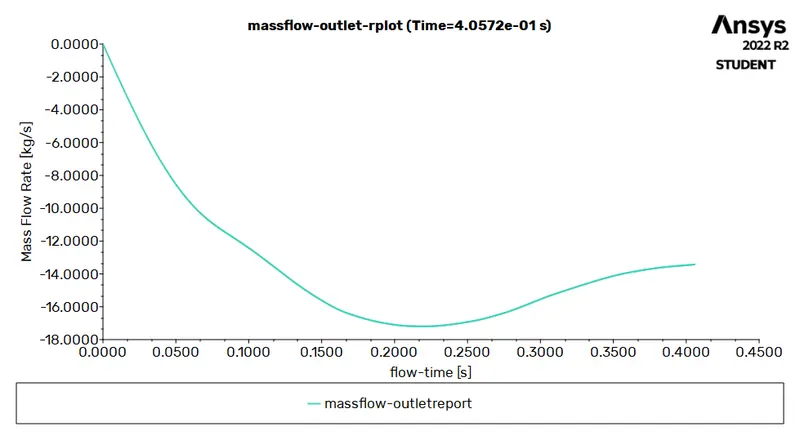
The image below shows the convergence of the mass flow rate at the outlet.
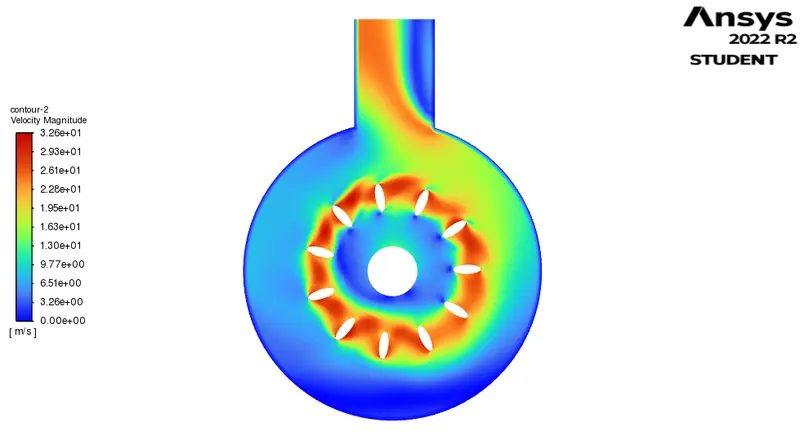
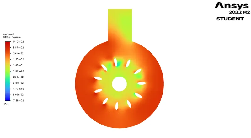
The images below show the instantaneous velocity and pressure distribution at T=0.4s.
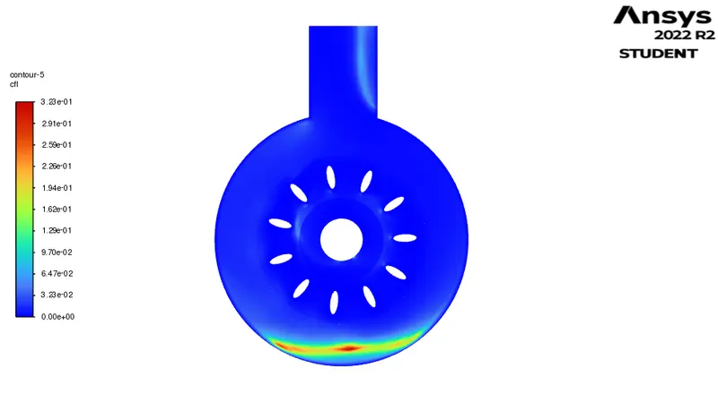
The image below shows the typical CFL number in the domain.
The drive link to the animated velocity distribution is attached below:
https://drive.google.com/file/d/1ZwV79q_PXisxZh9bftXPH6kGZG2Vjmr9/view?usp=sharing
From the video, it can be established that the flow field achieved a steady state after the first revolution.
Conclusion
The motion of the blades in the given generic turbomachinery component was simulated using the moving mesh unsteady approach. The blades were simulated at an rpm of 300 for about two full revolutions. The CFL number was maintained below 1 in the entire domain.