Week 4.1 - Genetic Algorithm

Aim

To find the global maximum of the stalagmite function by optimisation using Matlab. 

Introduction to Stalagmites and the stalagmite function

Stalagmites are rock formations commonly observed in cave floors rising upwards. These are created from the accumulation of material deposits dripping from the ceilings of the cave.

Mathematically, the shape of these stalagmites can be created using the stalagmite function as follows: 

`f(x,y) = f_{1x} * f_{2x} * f_{1y} * f_{2y}`

where, 

`f_{1x} = [sin(5.1pix + 0.5)]^6`

`f_{1y} = [sin(5.1piy + 0.5)]^6`

`f_{2x} = exp[-4*ln2*((x-0.0667)^2)/0.64 ]`

`f_{2y} = exp[-4*ln2*((y-0.0667)^2)/0.64 ]`

Introduction to the Genetic Algorithm

The genetic algorithm is an optimisation strategy inspired by natural selection in evolution to find the global minimum of a function. The genetic algorithm has 4 main phases to optimise the given function [1]. 

1. Initialization phase:
   The initial population is generated ensuring a full range of possibilities. This initial population can also be adjusted to be within key areas where the optimal solution is most likely to exist.
   
   
2. Selection phase:
   The individual solutions are selected based on the fitness function. Solutions that do not meet the fitness criteria are removed in the next iteration. 
   
   
3. Genetic Operations phase:
   The next generation of solutions is generated from the previously selected solutions by crossover and mutation mechanisms. 
   
   The crossover mechanism uses the information from two parent solutions to generate the next generation. 
   
   The mutation mechanism modifies the solution information of one parent to generate the next generation. This is required to ensure the optimisation does not converge prematurely and result in local minima.
    
4. Termination:
   This generational process is repeated until the termination condition is reached which can be:

• Solution satisfies minimum criteria
• Fixed number of generations reached
• The highest fitness solution reached, new generations do not produce better results

Syntax of Genetic Algorithm GA

The ga function is predefined in Matlab and has the following syntax [2]:

[x, fval] = ga(fun,nvars,A,b,Aeq,beq,lb,ub,nonlcon,options)

x - is the optimised global minima

fval - is the value of the fitness function at x

fun - is the function needing optimisation. (In this case, the stalagmite function). 

nvars - is the number of design variables as input to the function. 

A, b - are used to define the linear inequalities

Aeq, beq - are used to define the linear equalities

lb, ub - are used to define the lower and upper bounds of the design variables

nonlcon - is used to find the minima based on the constrains in nonlcon

options - minimisation process can be altered from the default settings by adjusting the options using optimoptions function. This is used in this case to increase the population size to 170 from the default 50. 

Strategy to arrive at a consistent solution using GA

The ga function uses random data to generate its population pool to determine the global minima. It is therefore important to check the consistency of the solution by looping the GA for multiple iterations and comparing the end results. To improve consistency with the results, a step-by-step approach is taken by introducing lower/upper bounds and increasing population size of the GA. 

Results

Study 1:

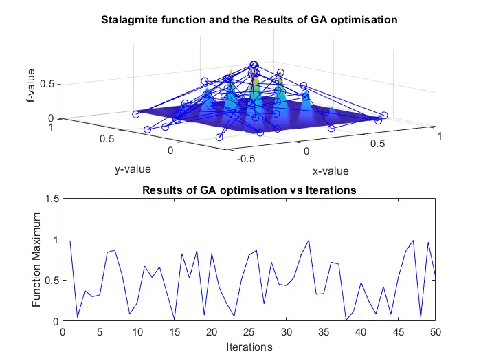
The figure below shows the first study of the Stalagmite function using GA. No lower/upper bounds were used and the population size was kept at default 50. The GA was run for 50 iterations and the solutions are shown to be erratic across the stalagmite function. The results of this optimisation are hence incorrect and inconsistent.

Study 2:

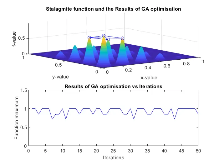
The figure below shows the second study of the stalagmite function using GA. This study introduced lower and upper bounds of the design variables to seed reasonable solutions for optimisation. The GA was run for 50 iterations and the results are seen to be more accurate and consistent compared to the previous study. Further study is required as there are still inconsistencies and inaccuracies in the results.

Study 3:

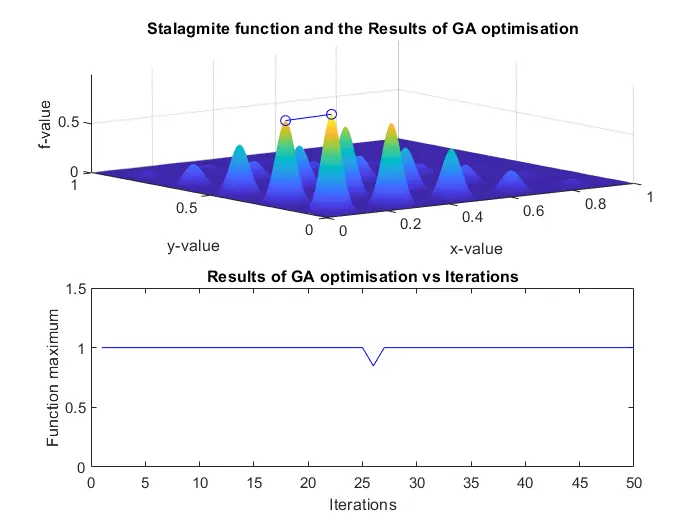
The figure below shows the third study of the stalagmite function using GA. This study increased the population size to 170 from the default 50 and maintained the lower and upper bounds of the design variables from the previous study. The GA was run for 50 iterations and the results are seen to be more accurate and consistent compared to the previous study. Further study is required as there are still inconsistencies and inaccuracies in the results.

Study 4:

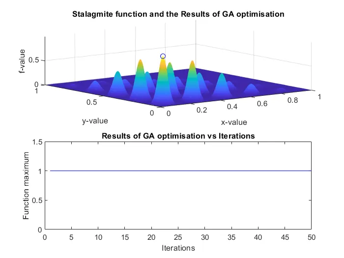
The figure below shows the fourth study of the stalagmite function using GA. This study narrowed down the lower and upper bounds and maintained the population size at 170 from the previous study. The GA was run for 50 iterations and the results are now accurate and consistent across all iterations. The results of this study can now be deemed optimised. 

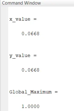
Global maxima of the stalagmite function:

Code:

Main

%% Optimization using Genetic Algorithm
clear all 
close all
clc
%% Inputs to create Stalagmite surface plot

x = linspace(0,1,200);
y = linspace(0,1,200);

%% 2D Mesh
[xx,yy] = meshgrid(x,y); % Generates a grid based on x and y arrays.

%% Evaluating Stalagmite function for surface plot

for i = 1: numel(xx(1,:))
    for j = 1:numel(yy(1,:))
        input(1) = xx(i,j);
        input(2) = yy(i,j);
        f(i,j) = stalagmite(input);
    end 
end

%% Optimisation using GA

%% Study1: 

num_cases = 50; % Number of runs to check consistency of optimisation

for i=1:num_cases    
[inputs,fval(i)] = ga(@stalagmite,2); 
    xopt(i) = inputs(1);
    yopt(i) = inputs(2);
end

%Figure
figure(1)
subplot(2,1,1)
surfc(xx,yy,-f) % Surface plot of stalagmite function
shading interp  % Removes grid lines from surface plot
hold on
plot3(xopt,yopt,-fval,'-bo')
hold off
xlabel('x-value')
ylabel('y-value')
zlabel('f-value')
title('Stalagmite function and the Results of GA optimisation')
subplot(2,1,2)
plot(-fval,'-b')
axis([0 50 0 1.5])
xlabel('Iterations')
ylabel('Function Maximum')
title('Results of GA optimisation vs Iterations')

%% Study2: 

num_cases = 50;
for i=1:num_cases    
% Introduced Lower and upper bound for input values to seed reasonable 
% solutions for optimisation
    [inputs,fval(i)] = ga(@stalagmite,2,[],[],[],[],[0;0],[1;1]); 
    xopt(i) = inputs(1);
    yopt(i) = inputs(2);
end

%Figure
figure(2)
subplot(2,1,1)
surfc(xx,yy,-f)
shading interp
hold on
plot3(xopt,yopt,-fval,'-bo')
hold off
xlabel('x-value')
ylabel('y-value')
zlabel('f-value')
title('Stalagmite function and the Results of GA optimisation')
subplot(2,1,2)
plot(-fval,'-b')
axis([0 50 0 1.5])
xlabel('Iterations')
ylabel('Function maximum')
title('Results of GA optimisation vs Iterations')

%% Study3: 

options = optimoptions('ga','PopulationSize',170)
% Increasing initial population size to 170 from default 50
num_cases = 50;
for i=1:num_cases    
[inputs,fval(i)] = ga(@stalagmite,2,[],[],[],[],[0;0],[1;1],[],[],options);
    xopt(i) = inputs(1);
    yopt(i) = inputs(2);
end

%Figure
figure(3)
subplot(2,1,1)
surfc(xx,yy,-f)
shading interp
hold on
plot3(xopt,yopt,-fval,'-bo')
hold off
xlabel('x-value')
ylabel('y-value')
zlabel('f-value')
title('Stalagmite function and the Results of GA optimisation')
subplot(2,1,2)
plot(-fval,'-b')
xlabel('Iterations')
axis([0 50 0 1.5])
ylabel('Function maximum')
title('Results of GA optimisation vs Iterations')

%% Study4: 

options = optimoptions('ga','PopulationSize',170)
num_cases = 50;
for i=1:num_cases    
% Further narrowed down lower and upper bound to zone in on optimised solution     
    [inputs,fval(i)] = ga(@stalagmite,2,[],[],[],[],[0;0],[0.1;0.1],[],[],options);
    xopt(i) = inputs(1);
    yopt(i) = inputs(2);
end

%Figure
figure(4)
subplot(2,1,1)
surfc(xx,yy,-f)
shading interp
hold on
plot3(xopt,yopt,-fval,'-bo')
hold off
xlabel('x-value')
ylabel('y-value')
zlabel('f-value')
title('Stalagmite function and the Results of GA optimisation')
subplot(2,1,2)
plot(-fval,'-b')
xlabel('Iterations')
axis([0 50 0 1.5])
ylabel('Function maximum')
title('Results of GA optimisation vs Iterations')

%% Results of Optimisation: X, Y and Global Maximum
clc
x_value = inputs(1)
y_value = inputs(2)
Global_Maximum = -(fval(1))

Function:

%% Stalagmmite Function
function [f]= stalagmite(input_vector) 
f1X = (sin(5.1*pi*input_vector(1) + 0.5))^6;
f1Y = (sin(5.1*pi*input_vector(2) + 0.5))^6;
f2X = exp(-4*log(2)*((input_vector(1)-0.0667)^2)/0.64);
f2Y = exp(-4*log(2)*((input_vector(2)-0.0667)^2)/0.64);
f=-f1X*f1Y*f2X*f2Y; % negative sign to ensure GA finds global maximum
end

Explanation of Code: 

The Genetic algorithm is used to determine the global minima of a function. In this case, the global maxima is required therefore the function is modified by inverting using a negative sign. While displaying the results of the optimisation, the results are again inverted with a negative sign thereby undoing the previous inversion. This ensures the global maxima of the function is found with appropriate visualisation.

Main

Lines 5-9: Generation of inputs to generate stalagmite surface plot

Lines 10-12: Generate a grid based on input arrays

Lines 13-22: Evaluating stalagmite function based on the mesh grid generated. 

Lines 25- 53: Study 1 of GA

Line 27 - Defining the number of iterations for GA to run

Lines 29-33: Loop to run GA based on number of iterations

Lines 35- 53: Plotting results of study 1 using subplot. 

Lines 54- 82: Study 2 of GA

Line 56 - Defining the number of iterations for GA to run

Lines 57-63: Loop to run GA based on the number of iterations with lower and upper bounds defined. 

Lines 65- 82: Plotting results of study 2 using subplot. 

Lines 84- 112: Study 3 of GA

Line 86: Defining population size of GA using optimoptions function

Line 88- Defining the number of iterations for GA to run

Lines 89-93: Loop to run GA based on the number of iterations with lower and upper bounds defined as well as increased population size.

Lines 94- 112: Plotting results of study 3 using subplot. 

Lines 114- 143: Study 4 of GA

Line 116: Defining population size of GA using optimoptions function

Line 117- Defining the number of iterations for GA to run

Line 118-123- Loop to run GA based on the number of iterations with defined population size and narrowed lower and upper bounds

Lines 125- 142: Plotting results of study 4 using subplot. 

Lines 144- 148: Displaying results of Optimisation

Line 145: clc command to clear console window from clutter GA outputs.

 Line 148: Negative sign to ensure results are shown for maximum value

Function

Line 2: Definition of input and output arguments of stalagmite function

Lines 3-6: Estimation of the various parameters of the stalagmite function.

Line 7: Negative sign included to invert the stalagmite function, so ga can easily identify the global maxima.

Errors Faced

No noteworthy errors were faced during the making of the script.

References

1. https://en.wikipedia.org/wiki/Genetic_algorithm
2. https://in.mathworks.com/help/gads/ga.html