Challenge

Project 1 - Parsing NASA thermodynamic data

RRahul Rajan Sourirajan7 Aug 2022

Aim

To extract the 14 coefficients of different species from the given NASA thermal data and estimate each species' Specific Heat Capacity (Cp), Enthalpy (H) and Entropy (S) along with its molecular weight using Matlab.

File Parsing

File parsing is the process of reading data from a file, usually text, and transforming the contents into usable data for computation and analysis. In this case, the Thermal data from NASA contains the coefficients to estimate the specific heat capacity, enthalpy and entropy of about 53 species. In order to use the data for computation, file parsing needs to be done.

The equations used to estimate the respective quantities of specific heat capacity, enthalpy and entropy using the respective coefficients are given as:

`C_p = R(a_1 + a_2 T + a_3 T^2 + a_4 T^3 +a_5T^4)`

`H = RT(a_1 + (a_2 T)/2 + (a_3 T^2)/3 + (a_4 T^3)/4 +(a_5T^4)/5 + a_6 /T)`

`S = R(a_1 lnT + a_2 T + (a_3 T^2)/2 + (a_4 T^3)/3 +(a_5T^4)/4 + a_7)`

where,

R - Universal Gas Constant [J/K.mol]

`a_1 to a_7` - Coefficients of the respective species [-]

T - Temperature [K]

Method

The given data contains about 53 species with each its own temperature range and coefficients. In order to extract and store the data collected from the datasheet, the structure datatype is used. Structures aid the organisation of large data using containers called fields. In this case, each species from the datasheet is assigned to a particular field in the structure and the corresponding coefficients and temperature ranges and other details are stored within that field. Using this datatype ensures ease of management and avoids confusion when run by various users.

%Thermo Data NASA
clear all 
close all 
clc

%% Read Data File and create main directory for files
File = fopen('THERMO.dat','r'); %Reads the data file
mkdir Species_Thermal_Data  % Creates a new directory in the folder
cd Species_Thermal_Data\ % Changes current directory to the directory created

%Suppressing warning commands Specifically for the CH2(S) species
% As name is isnt Matlab friendly.
w = warning('query','MATLAB:handle_graphics:exceptions:SceneNode');
id=w.identifier;
warning('off',id);

%% Acquire Headers and Global Temperature Range
%Loop to acquire Header
Header{1} = fgetl(File); 

%Acquire Global Temperature Range
Global_Temp_Range = strsplit(fgetl(File),' '); %Splits string delimited by space.
Global_Temp_Low =  str2double(Global_Temp_Range{2}); % Stores data for LowTemp
Global_Temp_Mid =  str2double(Global_Temp_Range{3}); % Stores data for MidTemp
Global_Temp_High =  str2double(Global_Temp_Range{4}); % Stores data for HighTemp

%Loop to aquire remaining header lines
for i= 1:3
Header{i+1,:} = fgetl(File);
end 

%Creation of Structure
Species = struct; 

%% Acquire species Data 
for k = 1:53 %Runs for all elements in the data sheet

%Species Header 
Species_Header = strsplit(fgetl(File),{' ','\t'}); % Acquires and splits Header line of the species demilited by space and tab
SpeciesName = matlab.lang.makeValidName(Species_Header{1}); % Ensures the name read in file is converted to Matlab valid name
Species.(SpeciesName).Header = Species_Header; % Stores the header line in the struct within a field created with the name of the species 

%Acquire species Coefficients
Species_coeff = struct; %Structure to acquire species coefficients

%Loop to acquire species coefficients
for j = 1:3 % Runs for the three lines of coefficients
Line_no = strcat('Line',num2str(j)); % Generates the string Line no.#
Species_coeff.(Line_no) = fgetl(File); %Stores the read data from the line to the respective Line no.# Field
Coeff_location = findstr(Species_coeff.(Line_no),'E'); % Finds the locations of E in the string

for i=1:5 % No. of terms in line 1 and line 2
    if i == 1 %For first coefficient in lines 1,2,3
     a(j,i) = str2double(Species_coeff.(Line_no)(1:Coeff_location(i)+3));
     %Identification of coefficients, from first digit to three digits after E
    elseif j==3 && i==5 %Last line, 5th term doesnt exist, hence break is used to stop the loop.     
        break 
    else  % For all other coefficients in Lines 1,2,3
     a(j,i) = str2double(Species_coeff.(Line_no)(Coeff_location(i-1)+4:Coeff_location(i)+3));
     %Identification of coefficients, from fourth character in string of
     %the previous coefficient (ie first digit of current coefficient) to 
     %three digits after E
    end
end

at = reshape(a.',1,[]); %Reshape command to line up all the coefficients in a neat 1D array.

end
%Allocation of the respective low temperature coefficients
Species.(SpeciesName).LowTempCoeff = at(8:14);
%Allocation of the respective High temperature coefficients
Species.(SpeciesName).HighTempCoeff  = at(1:7);
end


%% Acquiring data for estimation
allSpeciesList = fieldnames(Species); %Acquires Field names from the Species Structure 

for i = 1:numel(allSpeciesList) %For all the species in the datasheet
a = Species.(allSpeciesList{i}).LowTempCoeff; %Allocation of lowtemp coefficent to variable
T_low = str2double(Species.(allSpeciesList{i}).Header{end-3}); %Acquiring local low temperature from species header line
b = Species.(allSpeciesList{i}).HighTempCoeff; %Allocation of hightemp coefficent to variable
T_high = str2double(Species.(allSpeciesList{i}).Header{end-2}); %Acquiring local mid temperature from species header line
T_mid = str2double(Species.(allSpeciesList{i}).Header{end-1}); %Acquiring local high temperature from species header line

%%Estimation of Cp, H and S 
R= 8.3144598 ; % Universal Gas Constant

Local_temp = linspace(T_low,T_high,200); %Linearly space out data points between local low and high temperature

for j = 1:numel(Local_temp) %Number of temperature data points
    
%Cp, H and S
% If loop to check if loop temperature is lower than mid temperature
if Local_temp(j) < T_mid 
Cp(j) = R*(a(1) + a(2)*Local_temp(j) + a(3)*Local_temp(j)^2+ a(4)*Local_temp(j)^3+ a(5)*Local_temp(j)^4);
H(j) = R*Local_temp(j)*(a(1) + (a(2)*Local_temp(j)/2) + ((a(3)*Local_temp(j)^2)/3)+ ((a(4)*Local_temp(j)^3)/4) + ((a(5)*Local_temp(j)^4)/5) + a(6)/Local_temp(j));
S(j) = R*(a(1)*log(Local_temp(j)) +a(2)*Local_temp(j) + ((a(3)*Local_temp(j)^2)/2) +((a(4)*Local_temp(j)^3)/3 + ((a(5)*Local_temp(j)^4)/4) + a(7)));
else % Else case if loop temperature is higher than or equal to mid temperature
Cp(j) = R*(b(1) + b(2)*Local_temp(j) + b(3)*Local_temp(j)^2+ b(4)*Local_temp(j)^3+ b(5)*Local_temp(j)^4);
H(j) = R*Local_temp(j)*(b(1) + (b(2)*Local_temp(j)/2) + ((b(3)*Local_temp(j)^2)/3)+ ((b(4)*Local_temp(j)^3)/4) + ((b(5)*Local_temp(j)^4)/5) + b(6)/Local_temp(j));
S(j) = R*(b(1)*log(Local_temp(j)) +b(2)*Local_temp(j) + ((b(3)*Local_temp(j)^2)/2) +((b(4)*Local_temp(j)^3)/3 + ((b(5)*Local_temp(j)^4)/4) + b(7)));
end 
end

%Folder Creation for the respective species in loop
mkdir(allSpeciesList{i})
cd (allSpeciesList{i})

% Figures 
LegendText = allSpeciesList{i}; %Text to display in legend
figure(1)
plot(Local_temp ,Cp,'-r','Linewidth',2,'DisplayName',LegendText)
grid on
grid minor
xlabel('Temperature [K]')
ylabel('Cp [J/K.Kg]')
title('Cp vs Temperature')
legend show
saveas(gcf,'Cp_vs_Temperature.png') %Saves the image window

figure(2)
plot(Local_temp,H,'-b','Linewidth',2,'DisplayName',LegendText)
grid on
grid minor
xlabel('Temperature [K]')
ylabel('Enthalpy [J]')
title('Enthalpy vs Temperature')
legend show
saveas(gcf,'Enthalpy_vs_Temperature.png') %Saves the image window

figure(3)
plot(Local_temp,S,'-k','Linewidth',2,'DisplayName',LegendText)
grid on
grid minor
xlabel('Temperature [K]')
ylabel('Entropy [J/K]')
title('Entropy vs Temperature')
legend show
saveas(gcf,'Entropy_vs_Temperature.png') %Saves the image window

cd .. %Goes to parent folder to iterate for the next species 

%% Estimation of Molecular weight
Elements = {'N','C','H','O','A'}; %Name of the elements to aid in matching strings
Atomic_weights = [14,12, 1, 16, 40]; %Atomic weights of the respective elements
SpeciesName = allSpeciesList{i}; %Allocates name of the species to variable
M = 0; % Initial Molecular weight
for p = 1:numel(SpeciesName) %Running for each character in the species name
    for q = 1:numel(Elements) % Running for each of the elements
        if strcmpi(SpeciesName(p),Elements{q}) %If case to check and compare the current character to the element in the loops
            M = M + Atomic_weights(q); % If match is identified, the respective atomic weight is added to the molecular weight
                if p1 % If the number is greater than 1
                        M = M + Atomic_weights(q)*(n-1); %The atomic weight of the element is added
                        %accordingly based on the number of atoms of the element in the species
                        end
                end        
        else
             M = M; % if current element does not match with the current character in the species
        end
    end
end
MolecularWeight = M; 
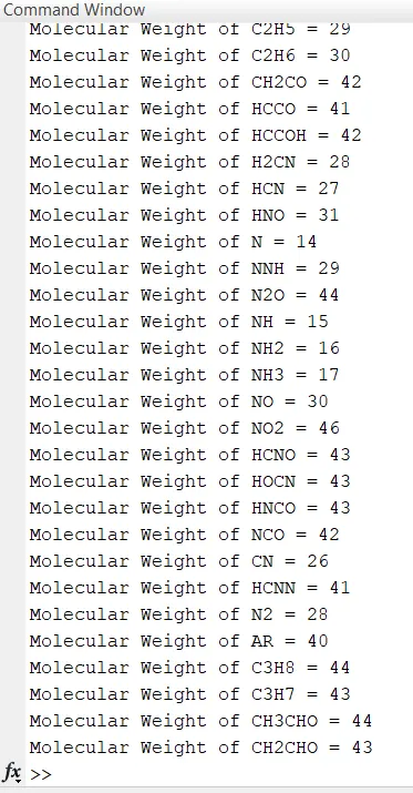
disp("Molecular Weight of " + SpeciesName + " = " + MolecularWeight); % Displays the molecular weight in the command window
end

The program is initialised by closing all open windows and clearing all data in the workspace and command window.
The next step reads the Nasa thermal data file. And creates a directory labelled as Species_Thermal_Data in the current folder and changes to that new directory.
The instance of CH2(S) species in the nasa thermal data is an invalid name in matlab, hence a command is used to convert that name to CH2_S_ by way of the make matlab.lang.makeValidName command. (This is shown in future steps). However with the changed name, the figure displays a warning indicating the text interpreter is unable to detect the syntax (due to the last underscore after S). This warning does not affect the working of the script, and hence is targeted and turned off, to avoid displaying in the command window.
The next step involves acquiring the headers and the global temperature range. This is done by using the fgetl command. A string split command is also used delimited by space to split and store the different values of temperature to low, mid and high respectively.
Another loop is created for 3 more iterations to obtain the remaining header lines and stored in the header variable.
The species structure is then created to organise and store all the data.
Loop is run 53 times to acquire data for all 53 species.
The first step in the loop acquires the respective header lines and split delimited by space and tab. The first string in the header line is the name of the species. the matlab.lang.makeValidName command is used to ensure all species names are valid within Matlab. (In this case, the CH2(s) species is modified to CH2_s_ by using this command). Without doing so, will cause an error and the program will stop. The species header and name now retrieved are stored within the species structure under its own species name.
A new structure is created to obtain the species coefficients.
Each species has three lines of coefficients with five terms in the first two lines and four terms in the third line (a total of 14 coefficients). In order to extract the coefficients, the lines are read in order and stored based on the respective line nos. This is done by the first loop running for 3 iterations.

The second nested loop runs for each coefficient within each line and extracts the coefficients. This is done by finding the location of E in the string and mapping the digits before and after to capture the complete coefficient.

In the code, the first if command checks if it's the first coefficient in the line. This acquires the first coefficient
starting from the first character to 3 characters behind E.
The next elseif command checks if it's the third line and 5th term and calls for a break in the loop, as there is no 5th term in line 3. The last else command acquires all the remaining coefficients. This is done by using the location of E and acquiring starting from 4 characters behind the previous coefficient's E location to 3 characters behind the current E location.
The data from the coefficients are now reshaped into a neat 1D array which is easier to visualise and compute.
Finally, the data from the 1D array is now stored in the low/High Tempcoefficients field in the respective species container of the structure.
The loop for 53 species ends here and at end of this loop, the structure will now have all the appropriate species' names and coefficients along with their header lines.
A new variable is created to store the names of the different species from the structure.
A new loop is started running for all the species in the list to compute their Cp, H and S.
The low/high temperature coefficients are stored in variables a and b, while the low, mid and high temperature values are retrieved in the header line of the species, based on their position from the end.
The universal gas constant is defined and the local temperature variable is created which contains 200 linearly spaced data points between low and high temperatures.
A nested loop is created for the total number of data points, to estimate Cp,H and S at each data point. An if command is used to check if the current temperature data point is below the mid temperature value. This ensures the usage of low temperature coefficients when this command is satisfied. The following else command ensures high temperature coefficients are used for all temperature data points greater than the mid temperature value.
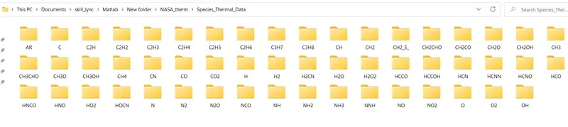
Folders are created based on the name of the current species in the loop, followed by a directory change.
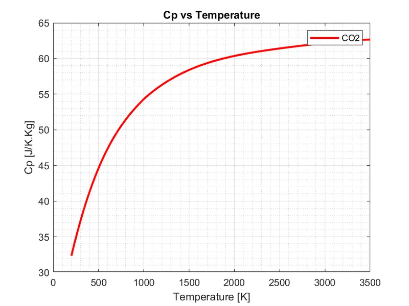
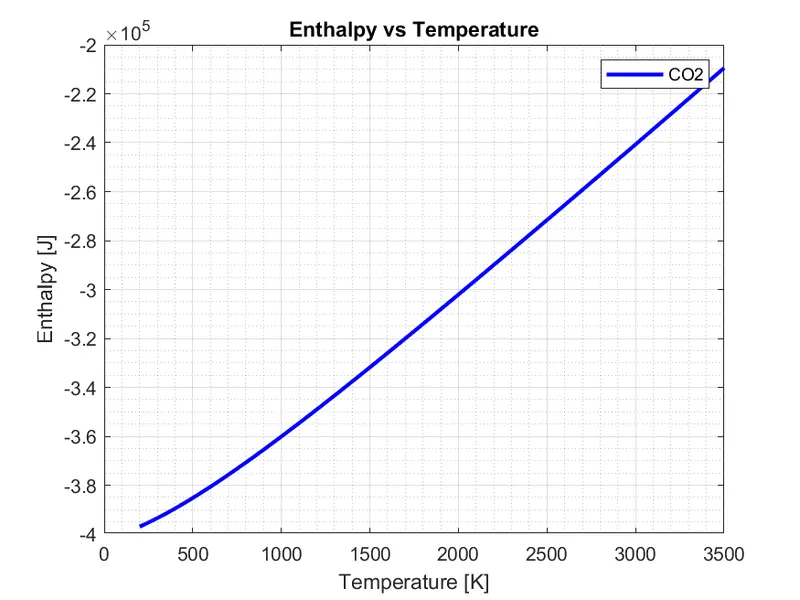
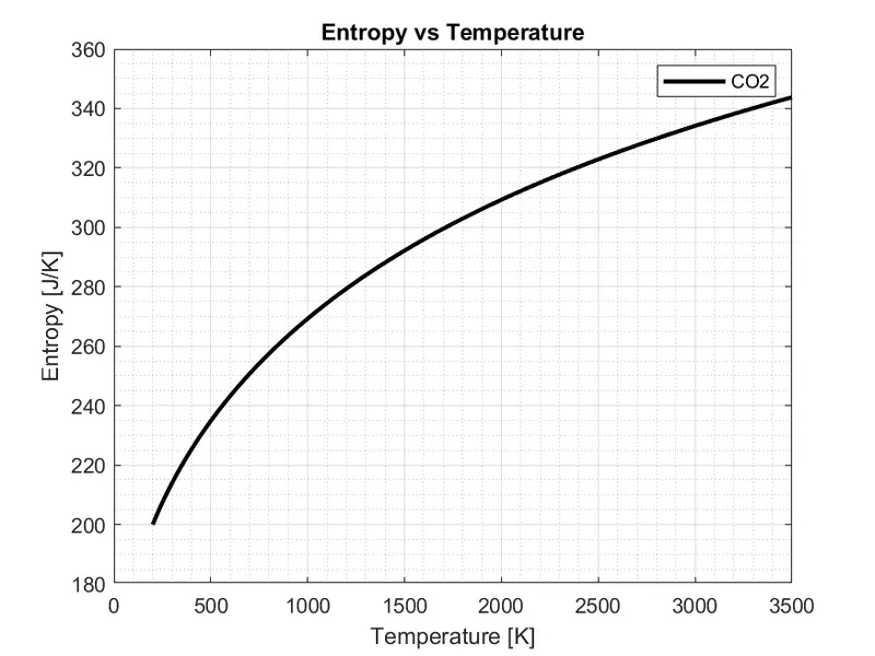
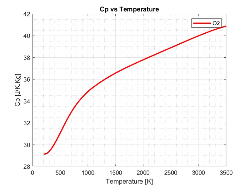
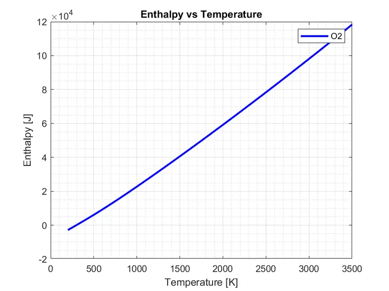
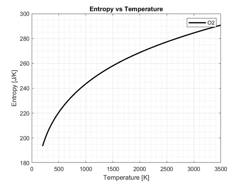
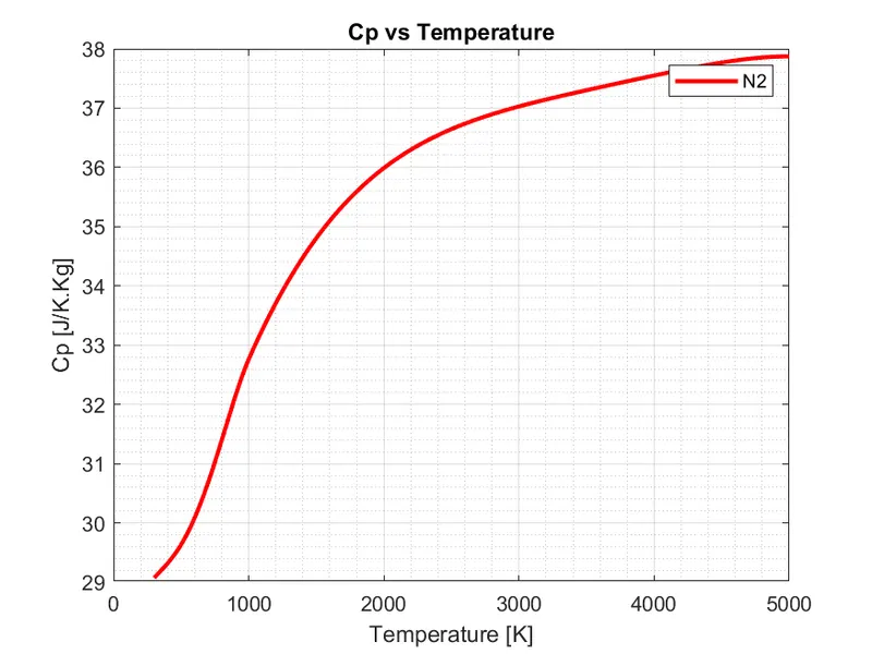
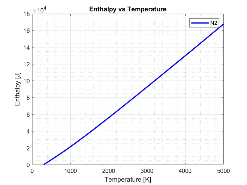
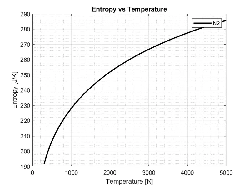
Figures are plotted for Cp vs T, H vs T and S vs T with legends displaying the name of the current species. The saveas command at end of figure line captures the window and saves it as an image in the folder created.
Once all images are created and saved, the cd.. command is used to go back to the parent folder.
To estimate the molecular weight, the elements are first defined to match and compare with the species' names. The respective atomic weights of the elements are also defined.
The molecular weight is initialized to zero for each species. A loop is run for all characters in the species name. A second nested loop is run for each of the elements. The if command compares the characters from the species to the element based on the current loops. If a match is found, the atomic weight of that element is added to the molecular weight. A second if command is used to check if the current character is before the last character of the string. If satisfied, the next character in the string is converted to a number (if that character is a number). The next if command checks if the number is greater than 1 (essentially identifying if number or character), and proceeds to multiply the atomic weights of that element based on the number. when the current element does not match with the current character in the species, the else command maintains the value of the molecular weight as before.
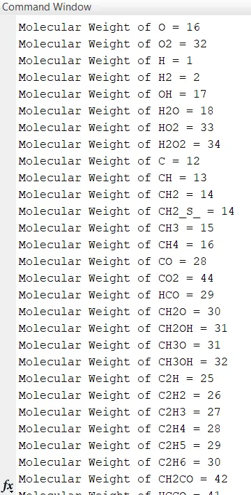
Finally, the molecular weight is displayed in the command window.