Week 1- Mixing Tee
Aim
To determine the mixing effectiveness of a mixing Tee with hot and cold inlets at `36^circ`C and `19^circ`C respectively with varying Momentum ratios and pipe length. Further, Compare the K-Epsilon and K-omega SST turbulence models for the given application.
Method
The mixing Tee is a common device used in various chemical applications where diffusion is of primary importance. It consists of two inlet pipes fixed at right angles to each other with an outlet aligned with one of the inlets. The fluids that need to be diffused with each other are passed in from the respective inlets and allowed to mix at the Tee Junction in the middle of the pipe. After mixing, the fluids then pass out of the mixing tee at the outlet as a well-mixed fluid.
The current study is performed on two cases involving a short and a long pipe. Each of these cases is run for Momentum ratios of 2 and 4 where Momentum ratio = velocity at cold inlet/velocity at hot inlet.
Geometry
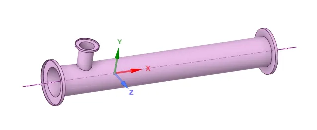
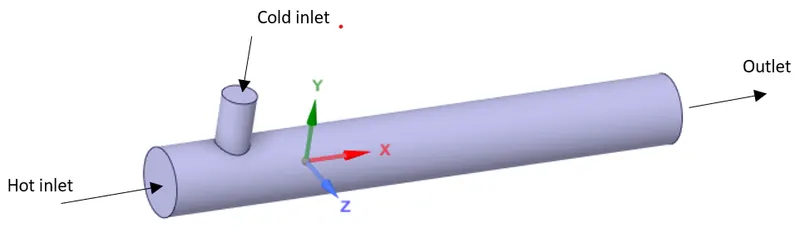
The outer geometry of the mixing-tee was provided as seen in the Figure below. The inner fluid volume of the geometry was then extracted and meshed to do the CFD Analysis.
Boundary Conditions
The boundary conditions applied for the various cases can be seen in the table below:
| Parameter | Short Pipe |
Long Pipe |
||
| MR 2 | MR 4 | MR 2 | MR 4 | |
| Cold Inlet Velocity | 6 m/s | 12 m/s | 6 m/s | 12 m/s |
| Hot Inlet Velocity | 3 m/s | 3 m/s | 3 m/s | 3 m/s |
| Cold Inlet Temperature | `19^circ`C | `19^circ`C | `19^circ`C | `19^circ`C |
| Hot Inlet Temperature | `36^circ`C | `36^circ`C | `36^circ`C | `36^circ`C |
| Outlet Guage Pressure | 0 Pa | 0 Pa | 0 Pa | 0 Pa |
Solver Setup
For this study, a steady-state pressure-based PV coupled scheme was employed. The fluid material used in this study was air. Continuity, momentum, energy and turbulence parameters were discretized using second-order upwind schemes. The solution was initialized using FMG initialization and run for a maximum of 300 iterations or until convergence was achieved. Convergence was monitored using scaled residuals and the solution is deemed converged when residuals of continuity reached 1e-5.
The K-omega SST and the Realizable K-Epsilon turbulence models were compared and the results are as follows:
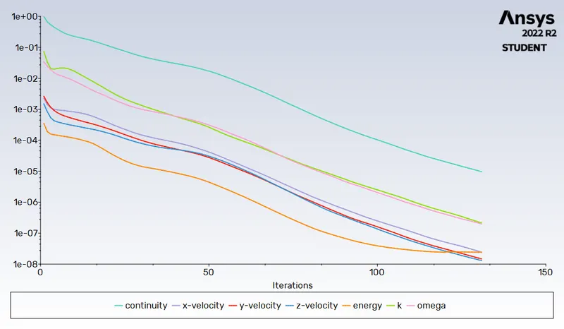
The image below displays the scaled residuals of the K-omega SST turbulence model. Residuals of continuity reached 1e-5 at 131 iterations.
The image below displays the scaled residuals of the Realisable K-Epsilon turbulence model. Residuals of continuity were not able to reach 1e-5 even at 300 iterations.
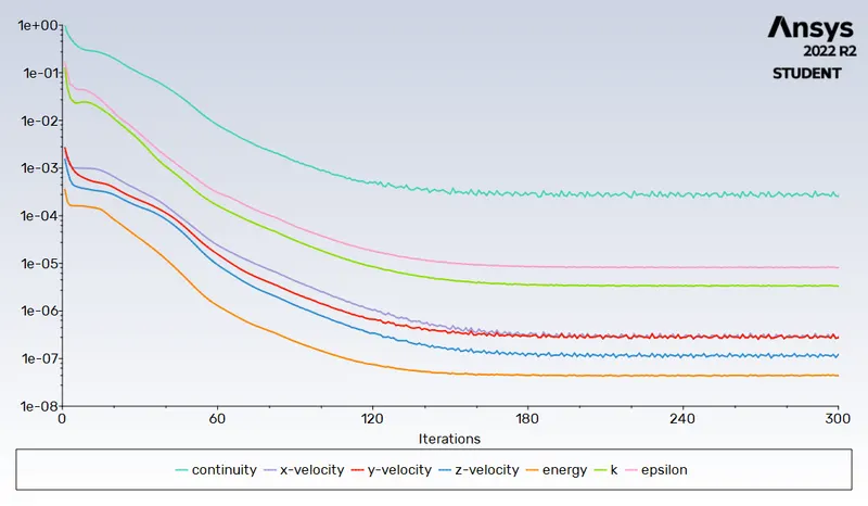
The k-omega SST turbulence model was thus chosen for all future simulations.
Mesh Sensitivity Analysis
A mesh sensitivity analysis was done to identify the variations in the results based on the mesh. To do so, three meshes were generated over the short pipe geometry with increasing mesh densities. All three meshes have 4 prism layers each with varying body cell sizings as seen below:
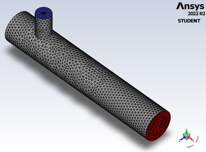
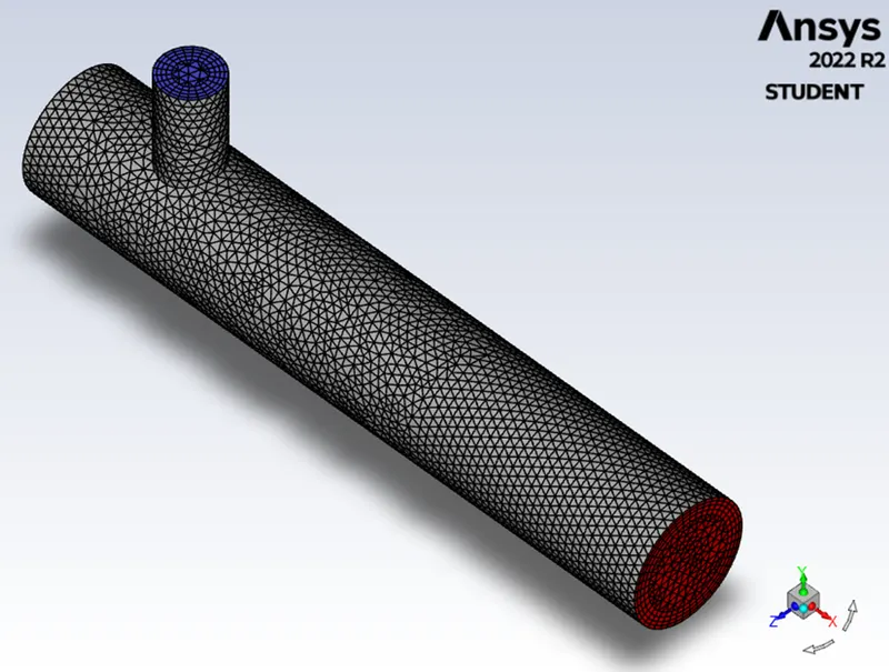
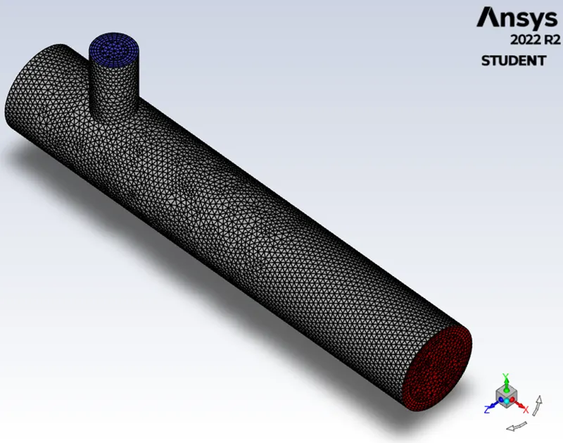
Mesh 1: 87k Nodes (3.2e-3m) Mesh2: 160k Mesh (2e-3m) Mesh 3: 300k Mesh (1.8e-3m)
The mesh sensitivity analysis was performed with the k-omega SST turbulence model.
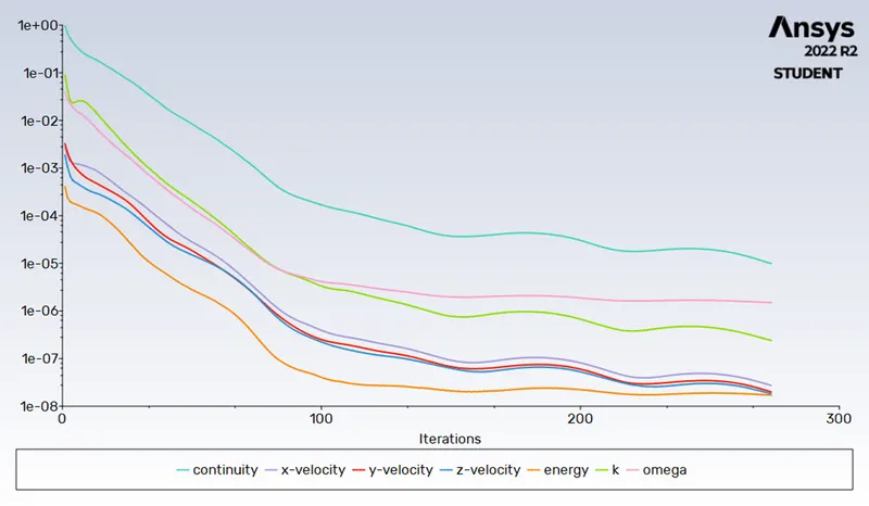
The image below displays the scaled residuals of Mesh 1 with 87k nodes. Residuals of continuity reached 1e-5 at 274 iterations.
The image below displays the scaled residuals of Mesh 2 with 160k nodes. Residuals of continuity reached 1e-5 at 131 iterations.
The image below displays the scaled residuals of Mesh 3 with 300k nodes. Residuals of continuity reached 1e-5 at 170 iterations and was continued to run to 225 iterations to allow residuals of continuity to reach 1e-6.
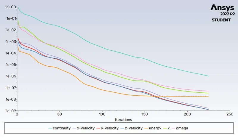
The table below displays the results of the Mesh sensitivity analysis:
| Mesh Size | Standard Deviation of Temperature at Outlet | Average velocity at Outlet | Standard Deviation of Velocity at Outlet | Iterations to Converge to 1e-5 for continuity |
| 87k Mesh | `1.10^circ`C |
6.02 m/s |
0.49 m/s | 274 |
| 160k Mesh | `1.33^circ`C | 6.04 m/s | 0.57 m/s | 131 |
| 300k Mesh |
`1.63^circ`C |
6.03 m/s | 0.66 m/s | 170 |
Mesh 2 with 160k nodes has values of the standard deviation of temperature and velocity at the outlet close to the higher density Mesh 3. Since the number of iterations to converge is lower for mesh 2 compared to mesh 3, Mesh 2 was thus chosen for all further simulations.
Results
Case 1: Short Pipe
Momentum Ratio 2
Velocity Contours across and along the pipe.
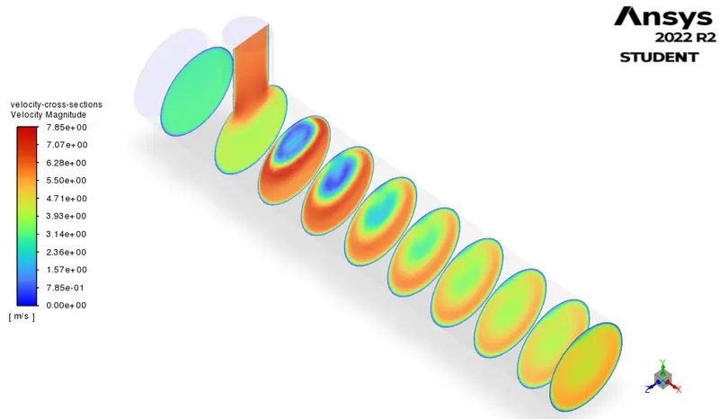
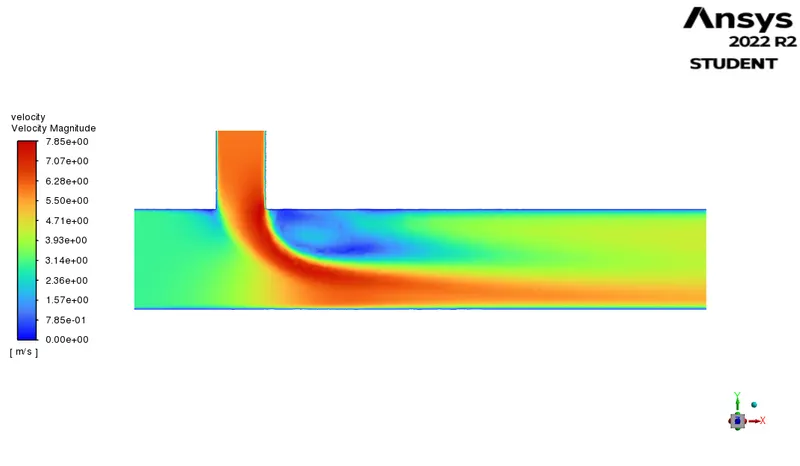
Temperature Contours across and along the pipe.
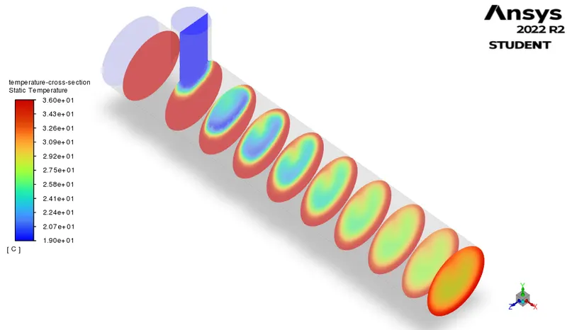
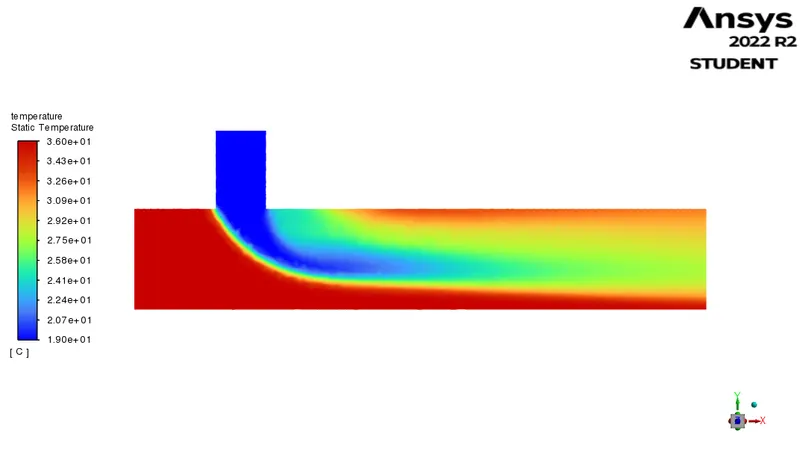
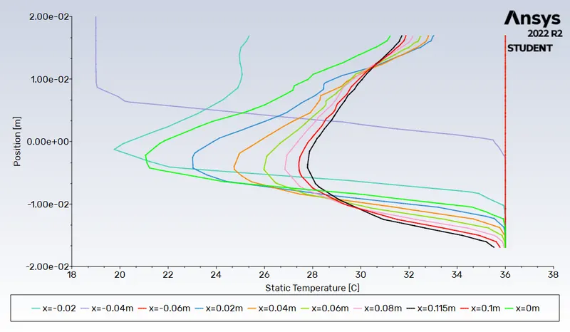
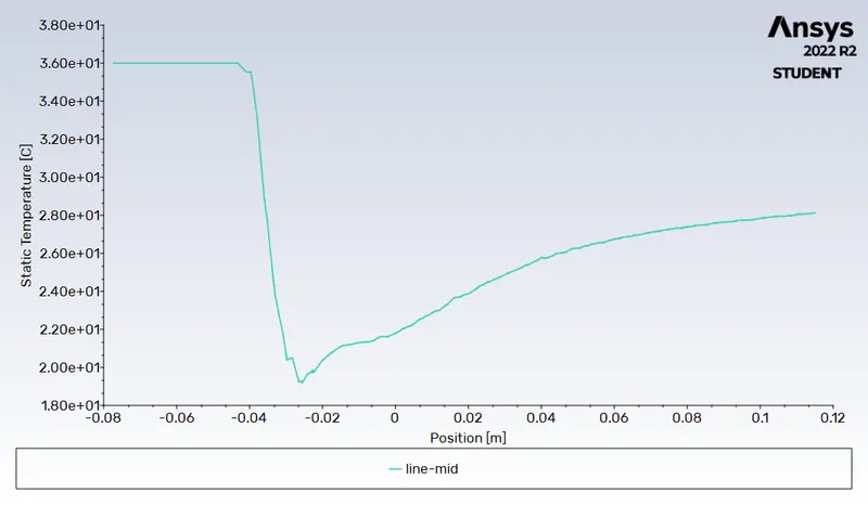
Temperature profiles across the pipe at various x locations and along the mid-line of the pipe.
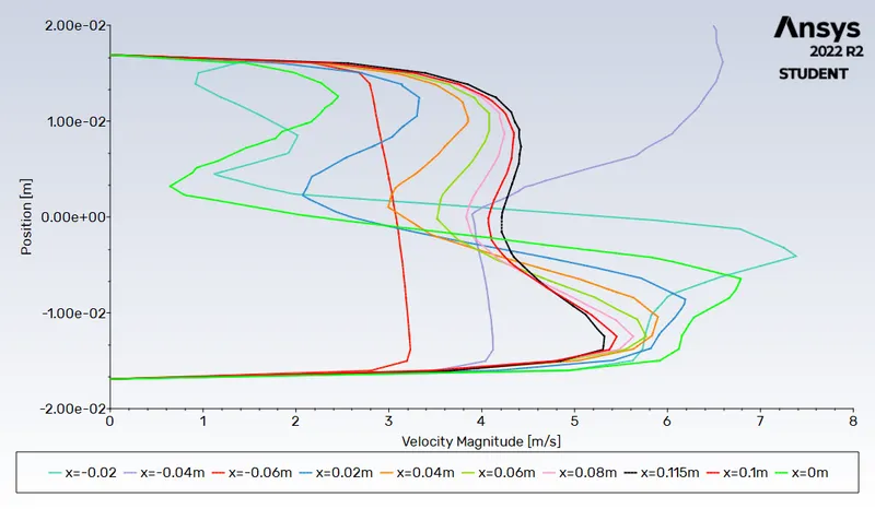
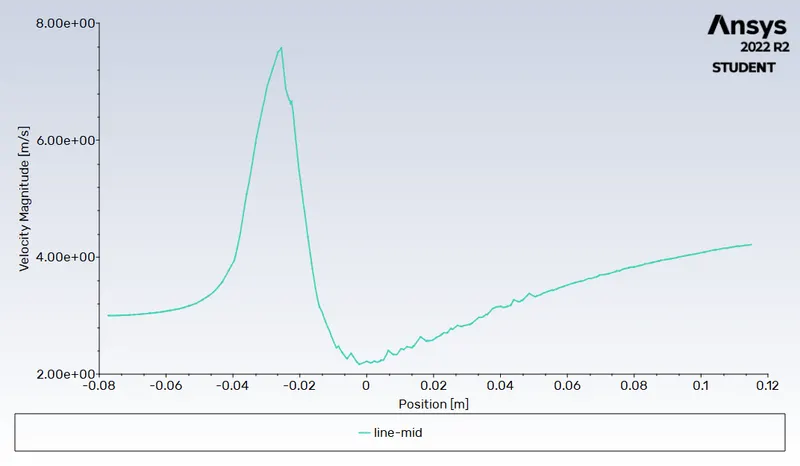
Velocity profiles across the pipe at various x locations and along the mid-line of the pipe.
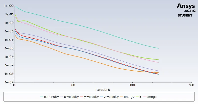
Scaled Residuals of continuity, momentum and energy
Momentum Ratio 4
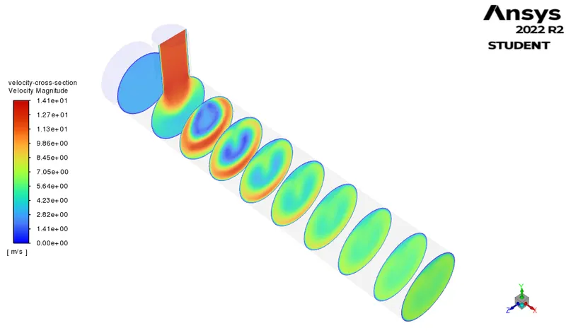
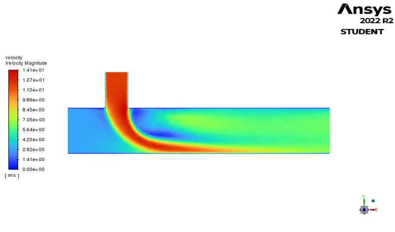
Velocity Contours across and along the pipe.
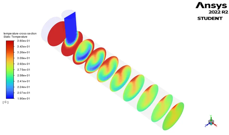
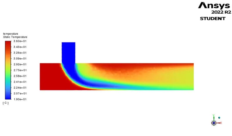
Temperature Contours across and along the pipe.
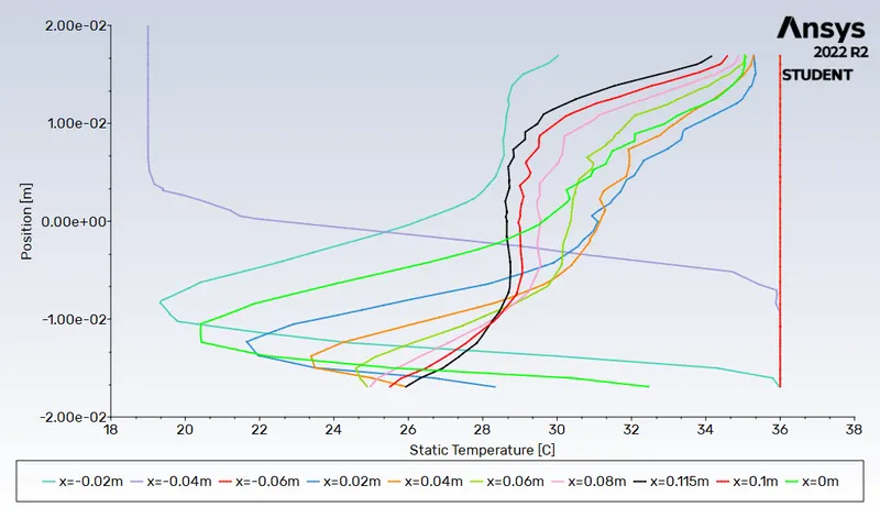
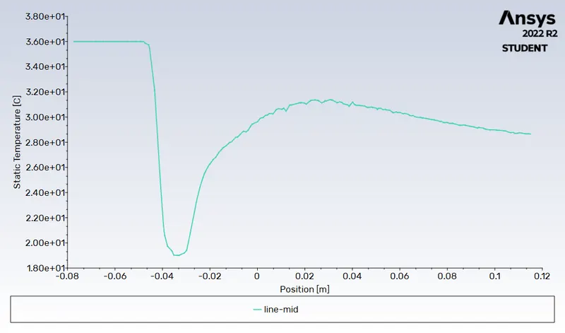
Temperature profiles across the pipe at various x locations and along the mid-line of the pipe.
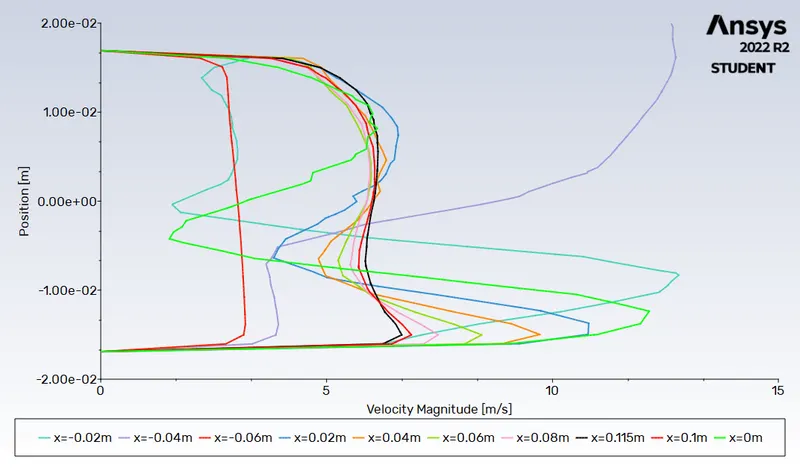
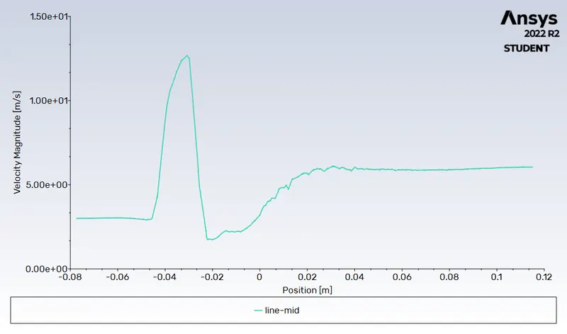
Velocity profiles across the pipe at various x locations and along the mid-line of the pipe.
Scaled Residuals of continuity, momentum and energy
Case 2: Long Pipe
Momentum Ratio 2
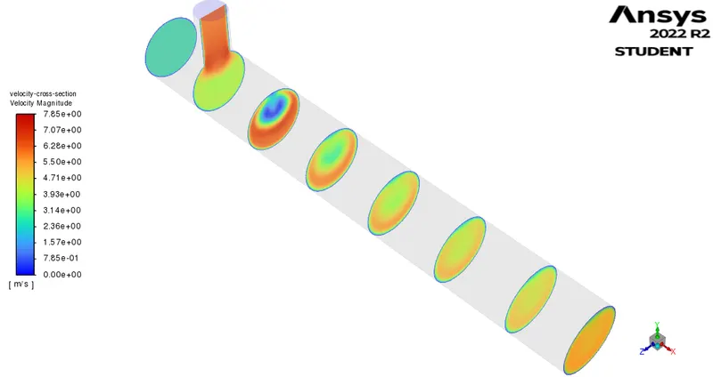
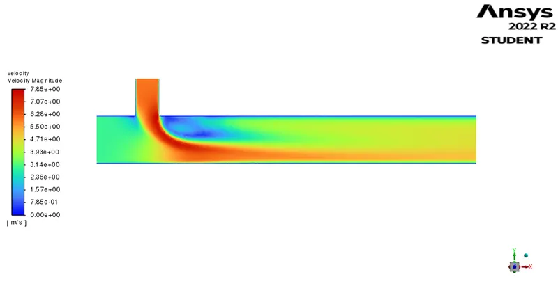
Velocity Contours across and along the pipe.
Temperature Contours across and along the pipe.
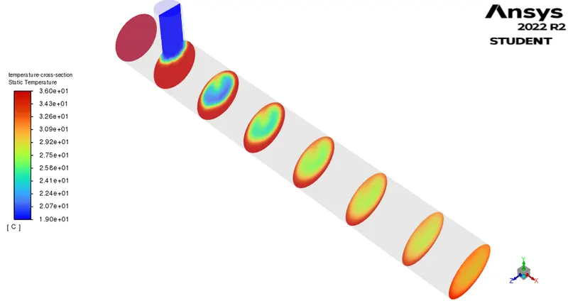
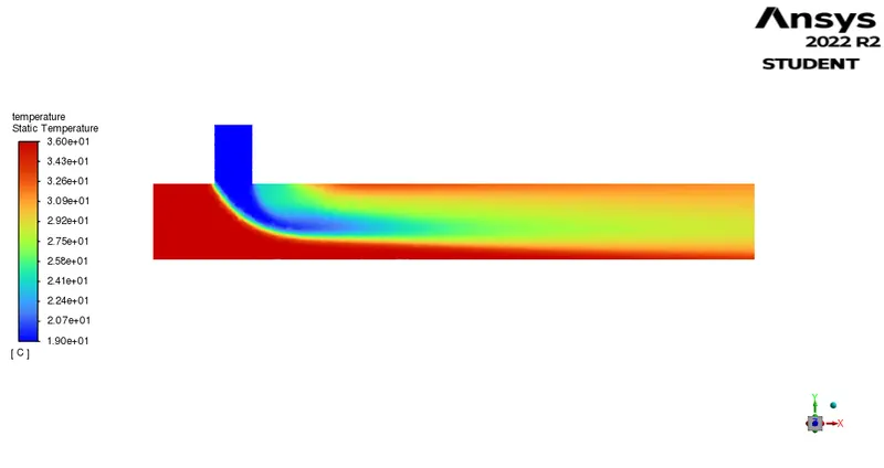
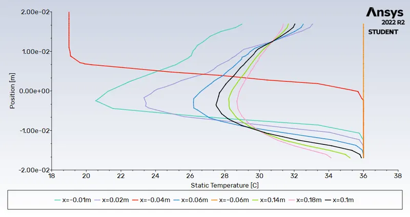
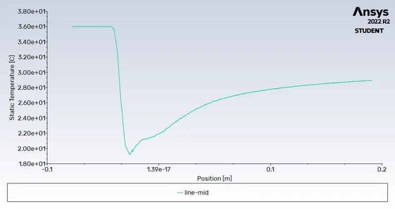
Temperature profiles across the pipe at various x locations and along the mid-line of the pipe.
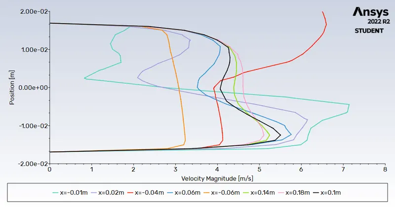
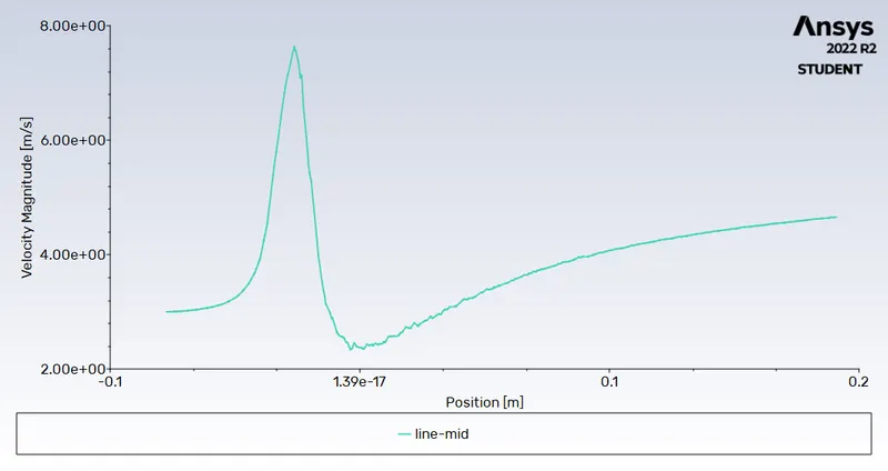
Velocity profiles across the pipe at various x locations and along the mid-line of the pipe.
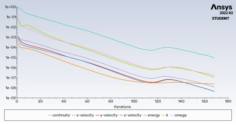
Scaled Residuals of continuity, momentum and energy
Momentum Ratio 4
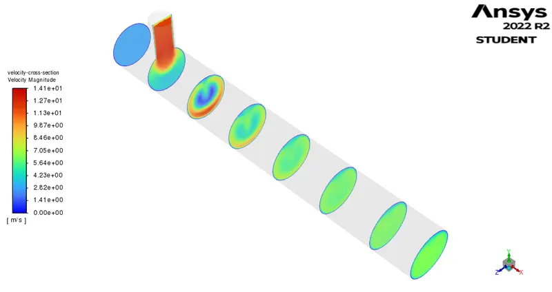
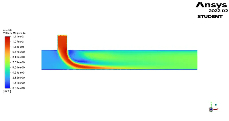
Velocity Contours across and along the pipe.
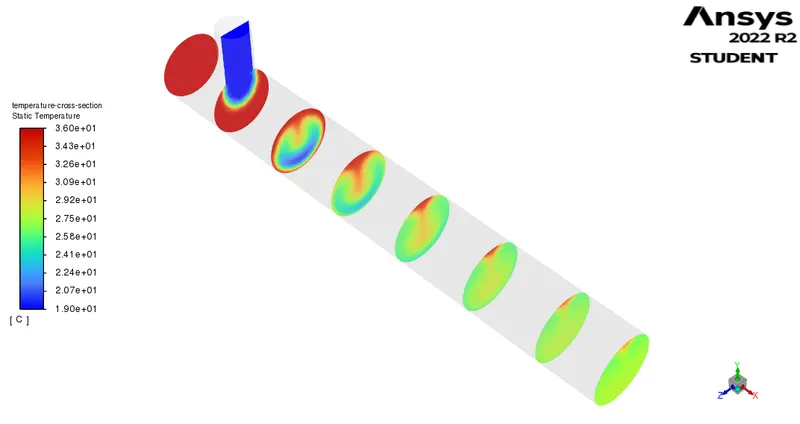
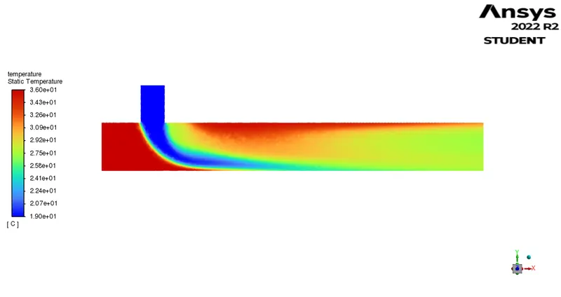
Temperature Contours across and along the pipe.
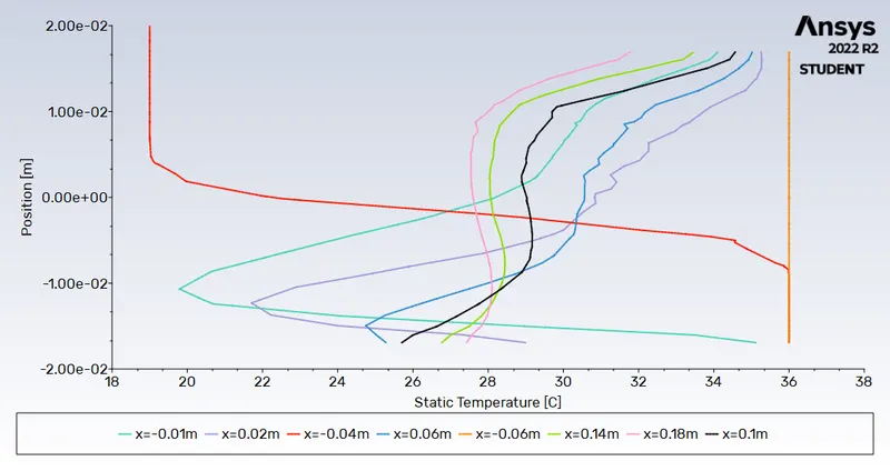
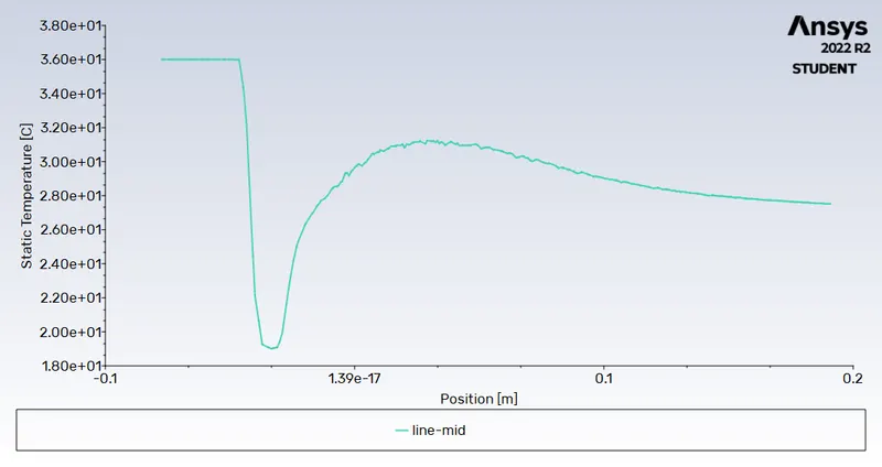
Temperature profiles across the pipe at various x locations and along the mid-line of the pipe.
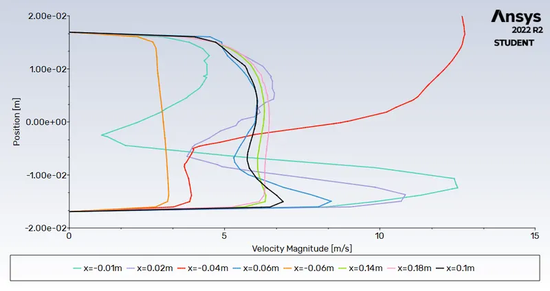
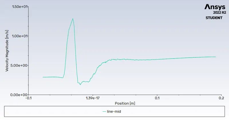
Velocity profiles across the pipe at various x locations and along the mid-line of the pipe.
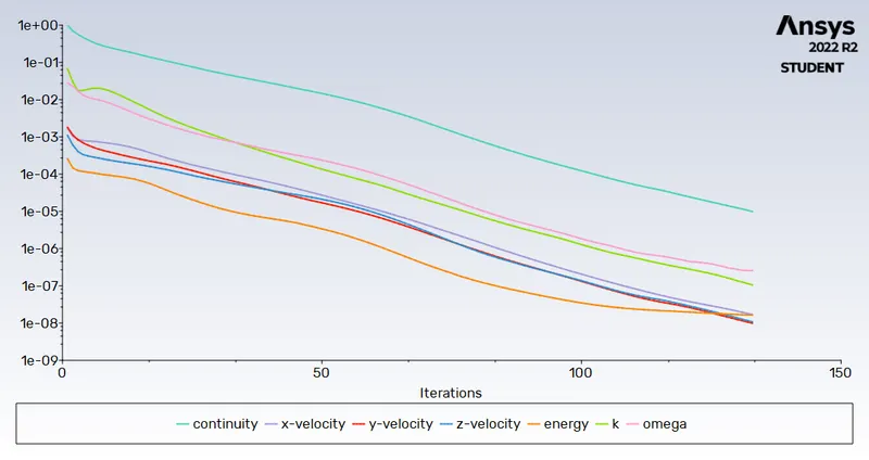
Scaled Residuals of continuity, momentum and energy
Comparison table of the two cases:
| Parameter | Short Pipe |
Long Pipe |
||
| MR 2 | MR 4 | MR 2 | MR 4 | |
| Cell Count | 160k | 160k | 220k | 220k |
| Average Outlet Temperature | `30.6^circ`C | `27.58^circ`C | `30.55^circ`C | `27.54^circ`C |
| Standard Deviation of Temperature at Outlet | `1.32^circ`C | `1.32^circ`C | `1.34^circ`C | `0.64^circ`C |
| Iterations to Convergence | 131 | 122 | 167 | 132 |
From the comparison table above, the length of the pipe does not seem to have a significant influence on the average outlet temperature. The increasing momentum ratio on the other hand drastically reduces the average outlet temperature. The standard deviation of temperature at Outlet however is much lower in the longer pipe with MR 4 indicating good mixing, this can be attributed to the increased time taken by the air to mix at higher velocities in the longer pipe.
Conclusion
From the study, it can be concluded that better mixing of hot and cold air can be achieved by using a longer pipe with a higher momentum ratio. Furthermore, increasing the momentum ratio also lowers the average temperature at the outlet.