Week 9 - Senstivity Analysis Assignment

Sensitivity analysis:

In a combustion process of fuel such as methane, there are lot of intermediatory reactions involved. In order to tune reaction mechanisms to match experimental conditions, the effect of each reaction on reactors dependent variables must be known. This is given in terms of sensitivity. First order sensitivity is defined as the rate of change of the independent varaible with respect to the dependent variable.

`W_(j,i) = (dZ_j)/(da_i)`

where, `W_(j,i)` -> first order sensitivity

`Z` -> reactor temperature and species mole fractions in reactor

`a` -> net reaction rate multiplier

Hence, sensitivity is given as a matrix with size number of reactions x number of variables

From this data, most influencial reactions can be obtained by choosing reactions that have largest sensitivity values for a particular variable of interest. Usually, temperature is chosen to be variable of interest, particularly when analyzing auto-ignition time delay.

In the current work, combustion of methane is performed using gri30 mechanism and the sensitivity of reactions are analyzed. Top few reactions that have highest sensitivity with respect to temperature are captured and listed out along with its sensitivity values. A python program is used for this exercise. A solution object is initialized to 1500 [k] temperature and 1 atm pressure. Stoichiometric amount of methane and air mole fractions are set to the object. An ideal gas constant pressure reactor is created using this object and added to reaction network. The reaction network advances the reactor to time-steps of 5e-6 [s] until 2e-3 [s]. During this time period the stoichiometric mixture auto-ignites and attains equilibrium. All the reactions in the reaction mechanism are used for sensitivity analysis. Among the reactions, top 10 reactions are picked and printed out in desending order after the simulation. The results are also plotted.

'''
Sensitivity analysis for methane combustion using Cantera
'''

import cantera as ct
import numpy as np
import matplotlib.pyplot as plt

# input variables
temp = 1500.0												# initial temperature
pres = ct.one_atm											# initial pressure
senst_parameter = "temperature"								# sensitivity parameter
no_senst_r = 10												# number of sensitive reactions considered
species_fraction = {"CH4":1,"O2":2,"N2":7.52}				# stoichiometric mixture of methane and air mole fraction
senst_reactions = {}										# result dict for top sensitive reactions

# initialize solution object with inputs, create ideal gas const 
# pressure reactor and assign it to reactor network
gas = ct.Solution("gri30.xml")
gas.TPX = temp, pres, species_fraction
r = ct.IdealGasConstPressureReactor(gas, name = "R1")
sim = ct.ReactorNet([r])

n_reactions = gas.n_reactions								# number of reactions in reaction mechanism
senst_factor = np.zeros(n_reactions)						# array to store max sensitivity for each reaction
states = ct.SolutionArray(gas,extra = ["t"])				# Cantera array to store solution states

# add all reactions to sensitivity analysis
for reaction in range(n_reactions):
	r.add_sensitivity_reaction(reaction)

# set relative and absolute tolerance for speicies convergence
sim.rtol = 1.0e-6
sim.atol = 1.0e-15

# set relative and absolute tolerance for sensitivity convergence
sim.rtol_sensitivity = 1e-6
sim.atol_sensitivity = 1e-6

for t in np.arange(0, 2e-3, 5e-6):
	# integrage reactor to a specified time-step of 5e-6[s] until 2e-3[s]
	sim.advance(t)
	states.append(r.thermo.state, t = 1000*t)
	for reaction in range(n_reactions):
		# for each reaction note down the max sensitivity factor during solution
		s = sim.sensitivity(senst_parameter,reaction)
		if abs(senst_factor[reaction]) < abs(s):
			senst_factor[reaction] = s

# sort reaction index in descending order of sensitivity factor
sorted_index_array = np.argsort(np.abs(senst_factor))[::-1]
# filter the sorted index array to obtain required number of top reactions
filtered_index_array = sorted_index_array[:no_senst_r]

for idx in filtered_index_array:
	# Update result array with reaction name and its sensitivity factor for top reactions
	senst_reactions[sim.sensitivity_parameter_name(idx)] = senst_factor[idx]

# print the results in table format
print("-"*60)
print("%-30s|%-30s" %(" Reaction"," Sensitivity"))
print("-"*60)
for key, value in senst_reactions.items():
	print("%-30s|%30s" %(key, value))
print("-"*60)

# plot evolution of temperature and other species
plt.figure(1)
plt.subplot(2,2,1)
plt.plot(states.t, states.T)
plt.title("temperature vs time[ms]")
plt.subplot(2,2,2)
plt.plot(states.t, states('OH').X)
plt.title("OH vs time[ms]")
plt.subplot(2,2,3)
plt.plot(states.t, states('H').X)
plt.title("H vs time[ms]")
plt.subplot(2,2,4)
plt.plot(states.t, states('CH4').X)
plt.title("CH4 vs time[ms]")
plt.tight_layout()

# plot the sensitivity for top reactions
plt.figure(2)
plt.barh(range(no_senst_r),list(senst_reactions.values())[::-1])
plt.yticks(range(no_senst_r),list(senst_reactions.keys())[::-1])
plt.grid()
plt.title(f"Sensitivity of top {no_senst_r} reactions")
plt.tight_layout()
plt.show()

Results:

Top reactions having largest sensitivity

------------------------------------------------------------
 Reaction                     | Sensitivity                  
------------------------------------------------------------
R1: CH3 + O2 <=> CH3O + O     |            16.835127519597958
R1: 2 CH3 (+M) <=> C2H6 (+M)  |           -13.608284614964061
R1: H + O2 <=> O + OH         |            13.093953803107844
R1: CH4 + H <=> CH3 + H2      |           -10.149715891890242
R1: CH3 + O2 <=> CH2O + OH    |             6.774938121903749
R1: CH3 + HO2 <=> CH3O + OH   |             6.265928293637251
R1: 2 CH3 <=> C2H5 + H        |             4.342079380642883
R1: CH2O + CH3 <=> CH4 + HCO  |             4.026016597217002
R1: CH2O + O2 <=> HCO + HO2   |             4.023307377567686
R1: CH3 + HO2 <=> CH4 + O2    |            3.4345346958183685
------------------------------------------------------------

Species Evolution:	Sensitivity analysis

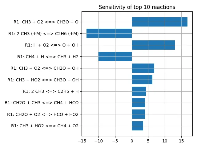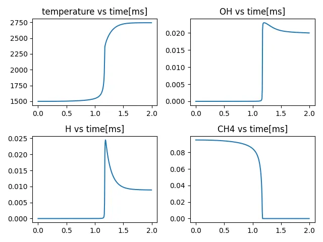
The table shows the list of top 10 reactions having large sensitivities for temperature. Some of the sensitivities are positive while others are negative. Postive sensitivity shows that the reactions help increase the temperature of reactor and hence reduce the auto-ignition delay. However negative sensitivities show that the reaction reduces the temperature in domain and hence increase the auto-ignition delay. Based on their sensitivities the amount of adjustment to a reaction coefficient can be adjusted to match the reaction mechanism to experimental conditions and results. The second plot shows the evolution of temperature and few species with time. Temperature stays nearly constant unitl 1 ms at which point the auto-ignition nearly starts. Temperature shoots up suddenly and reaches an equilibirum point. The species concentrations for OH and H also show similar behaviour.. After auto-ignition, they rise up sharply and drop to equilibrium levels. CH4 however starts to get consumed in small ratio before auto-ignition and the ratio drops suddenly after auto-ignition. The fuel completely burns out at equilibrium. The third chart showns the same table above in graphical format for better visualization of which reactions dominate the temperature change in the domain.