Week 9 - Parametric study on Gate valve.
GATE VALVE SIMULATION:
Objective:
In this challenge our objective is to perform parametric study on the gate valve by setting the opening from 10% to 80%.
Thereby we will obtain mass flow rates at the outlet for each opening point.
Calculate the flow coefficient and flow factor for each opening and plot the graph.
Discuss the results of the mass flow rate and flow coefficient.
Introduction:
Gate valve:
A gate valve, also known as a sluice valve, is a valve that opens by lifting a barrier (gate) out of the path of the fluid. Gate valves require very little space along the pipe axis and hardly restrict the flow of fluid when the gate is fully opened. The gate faces can be parallel but are most commonly wedge-shaped (in order to be able to apply pressure on the sealing surface).
Use:
Gate valves are used to shut off the flow of liquids rather than for flow regulation. When fully open, the typical gate valve has no obstruction in the flow path, resulting in very low flow resistance. The size of the open flow path generally varies in a nonlinear manner as the gate is moved. This means that the flow rate does not change evenly with stem travel. Depending on the construction, a partially open gate can vibrate from the fluid flow.
Gate valves are mostly used with larger pipe diameters (from 2" to the largest pipelines) since they are less complex to construct than other types of valves in large sizes.
At high pressures, friction can become a problem. As the gate is pushed against its guiding rail by the pressure of the medium, it becomes harder to operate the valve. Large gate valves are sometimes fitted with a bypass controlled by a smaller valve to be able to reduce the pressure before operating the gate valve itself.
Gate valves without an extra sealing ring on the gate or the seat are used in applications where minor leaking of the valve is not an issue, such as heating circuits or sewer pipes.
Gate valves are typically constructed from cast iron, cast carbon steel, ductile iron, gun metal, stainless steel, alloy steels, and forged steels.
The flow coefficient - Cv - or the flow factor - Kv - are commonly used to specify capacities of control valves.
Flow Co-efficient:
where
- Kv is the flow factor expressed in `m^3*h^(-1)`.
- Q is the flowrate (expressed in cubic metres per hour `m^3/h`,
- SG is the specific gravity of the fluid (for water = 1),
- ∆P is the differential pressure across the device (expressed in [Bar]).
Kv can be calculated from Cv using the equation:
- `K_v = 0.865*C_v`
Steps Followed:
a) Geometry preperation
b) Meshing
c) Setup
d) Results
The following steps will be followed in setting up the simulation in Ansys Fluent.
a) Geometry preperation:
Firstly, we will import the geometry in to the spaceclaim.
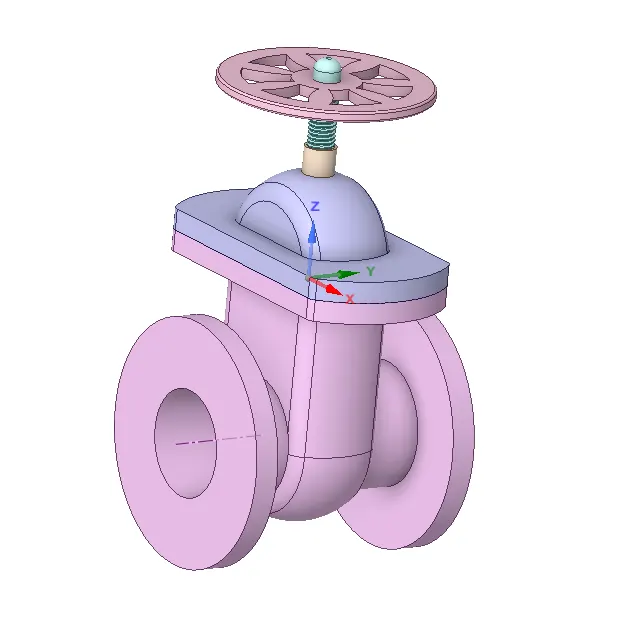
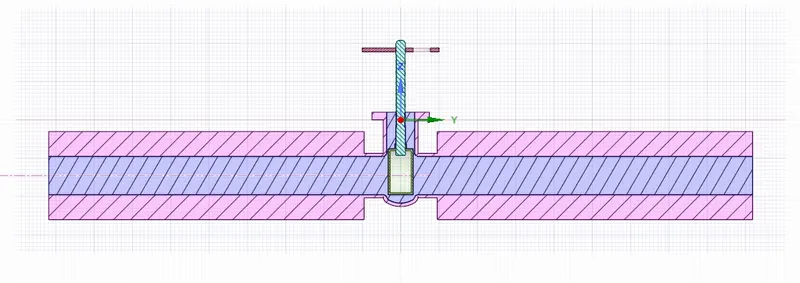
Move the disc by 10mm using the pull tool.
We can see small opening in the given figure.
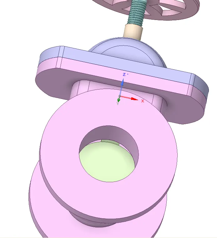
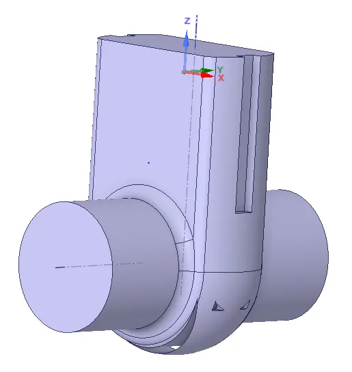
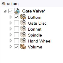
In Prepare use volume extract option, to extract fluid volume.
Using pull tool, extend inlet and outlet by 800mm.
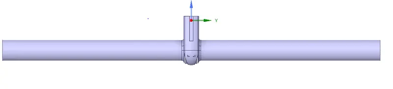
Suppress all the solid volumes.
b) Meshing:
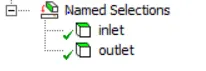
Create Named Selections
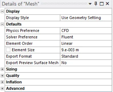
Basic Mesh:
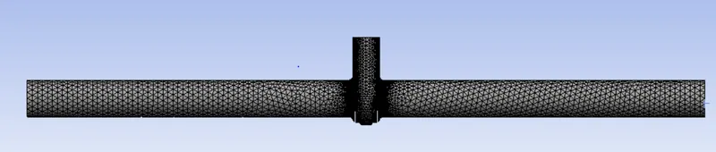
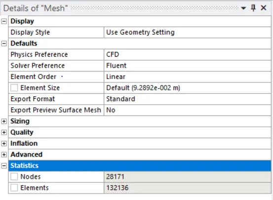
We will refined mesh for the simulation.
c) Setup:
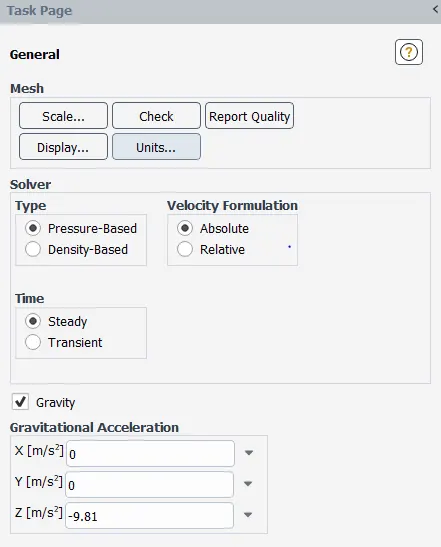
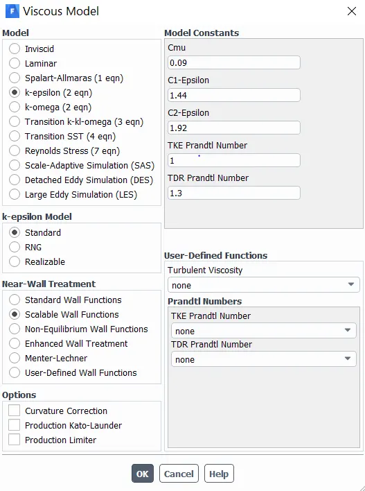
Following options are selected.
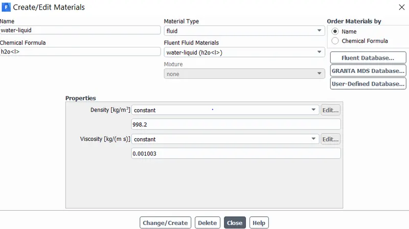
Materials:
Cell zones:
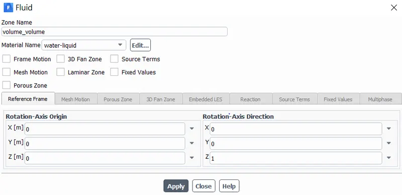
Boundaries:
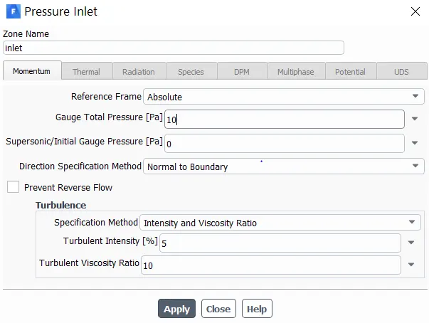
In solution > initialize the solution.
Definitions > mass flow rate at ooutlet.
In post-processing,
Create planes along the length of the pipe.
Create velocity and pressure contour.
In Solution > Create the velocity and pressure animations.
d) Results:
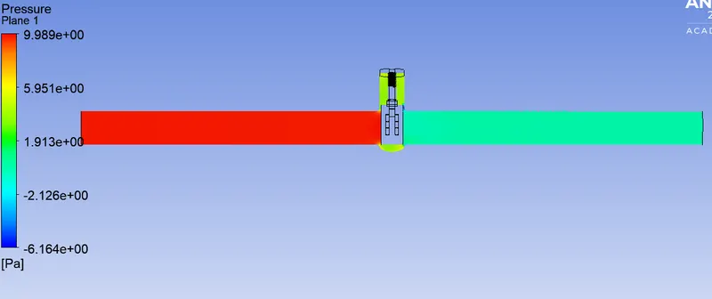
The following results were obtained with 10mm open.
Geometry:
Mesh:


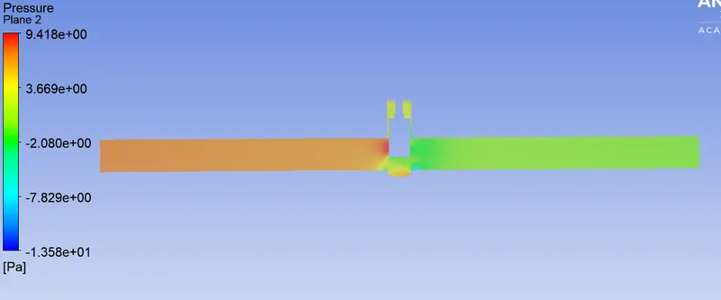
Pressure Contour:
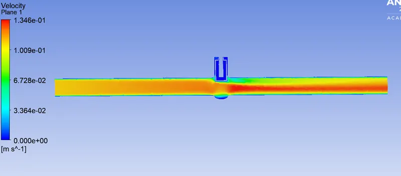
Velocity Contour:
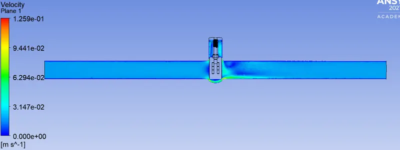
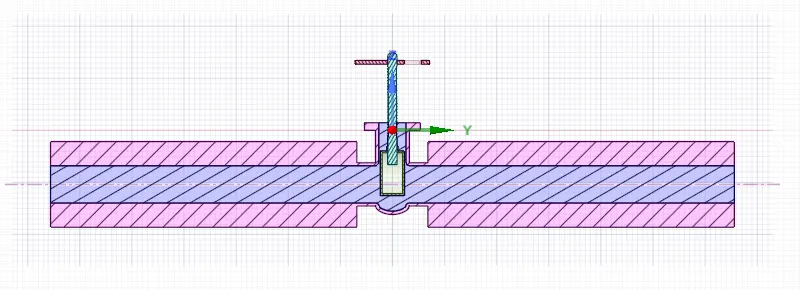
The following results were obtained with 30mm open.
Geometry:
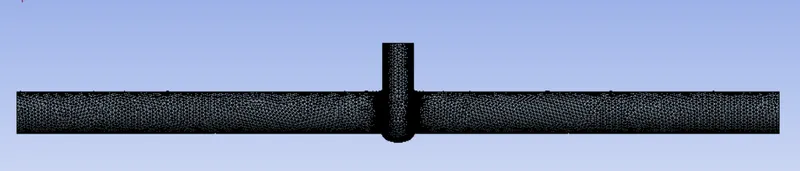
Mesh:

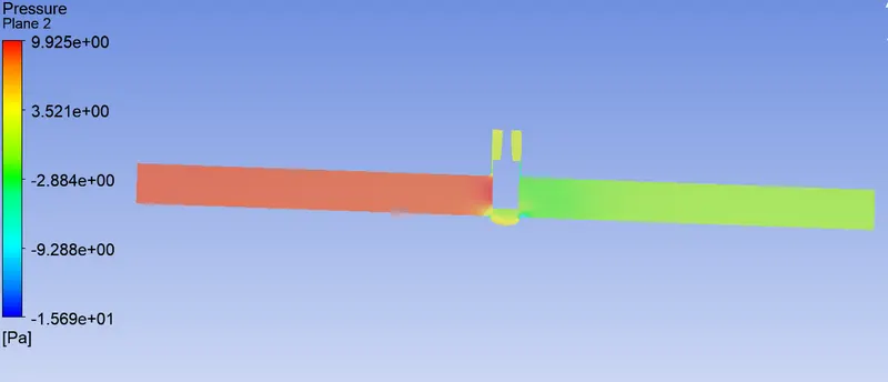
Pressure Contour:
Velocity Contour:
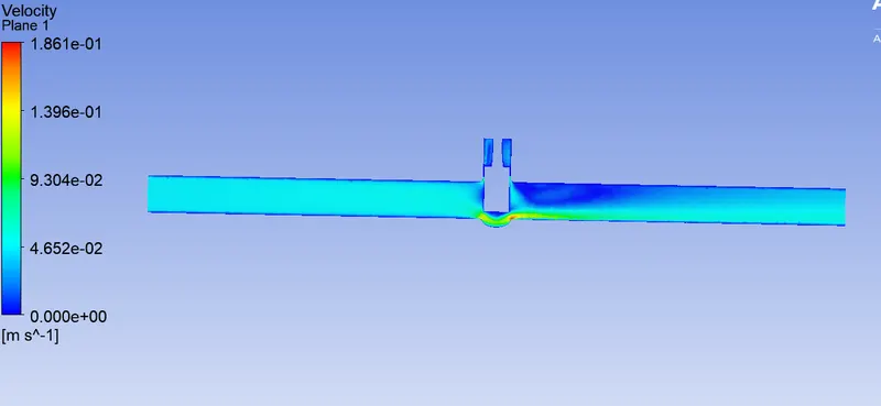
The following results were obtained with 50mm open.
Geometry:
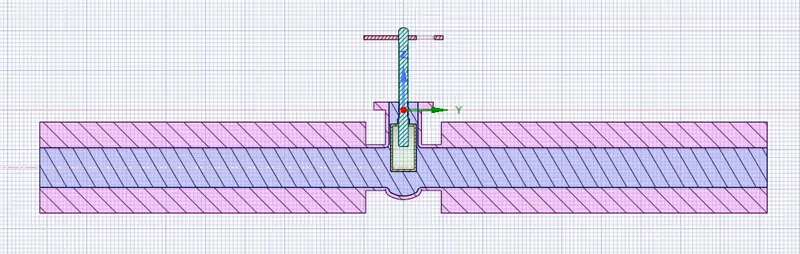
Mesh:
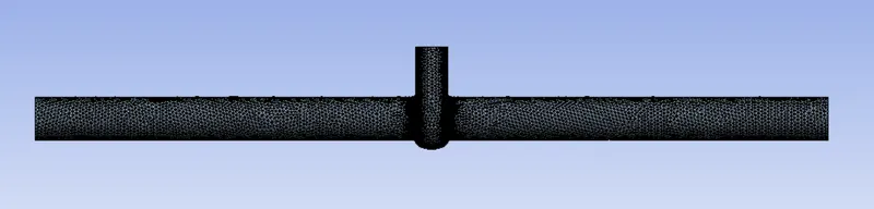

Pressure Contour:
Velocity Contour:
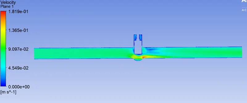
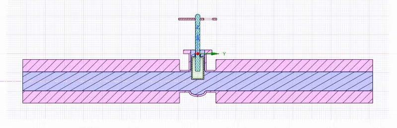
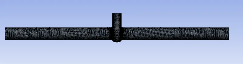
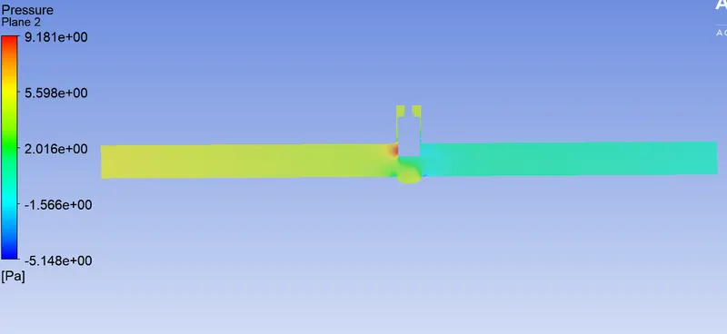
The following results were obtained with 70mm open.
Geometry:
Mesh:

Pressure Contour:
Velocity Contour:
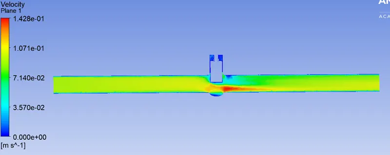
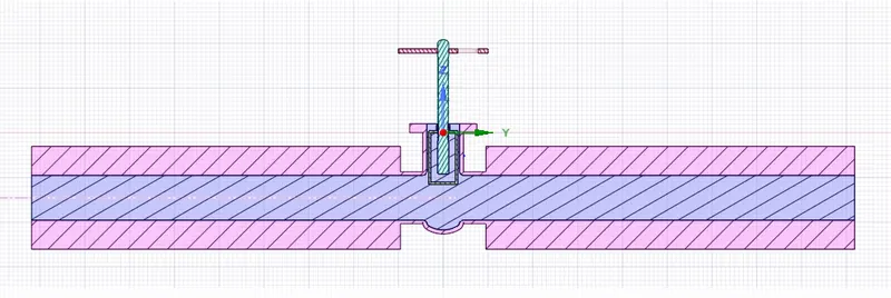
The following results were obtained with 90mm open.
Geometry:
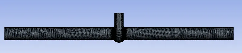
Mesh:

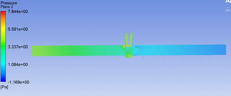
Pressure Contour:
Velocity Contour:
Conclusion:
The following table was obtained from the parametric study.
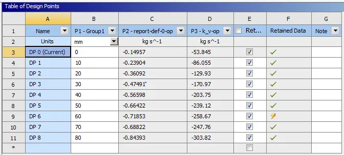
The mass flow rate at each opening of the valve are available in the parametric study table.
Graph between opening of the valve in mm and flow co-efficient.
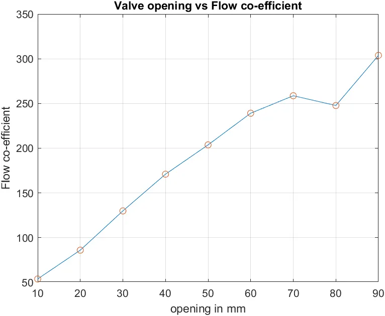
Smaller the valve opening, more the pressure loss and lesser the flow rate. We need to design the valve such that it has large value of the Flow co-efficient at operating conditions.