Week 9 - FVM Literature Review

Finite Volume Method(FVM):

Finite Volume Method is a discretisation method, used for approximation of partial differential equations. It is a method for evaluating and representing partial differential equations in the form of algebraic equations. The key step of the control volume is the integration of the governing equation over a small control volume to yield a discretised equation at its nodal point. Nodal point is the point with in the small control volume, which holds the average properties of the control volume.

There are three major steps followed in solving a differential equation using the finite volume method:

1.Generating grid

2.Discretisation of equation

3.Solving the system of algebraic equations

We will discuss briefly one by one, by using the 1-D linear heat conduction equation.

1. Generating grid:

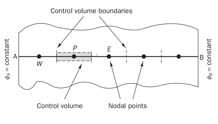
For solving any problem using numerical method, grid is required to split the domain into discrete elemetal domains. In the same way, finite volume methods divide the domain volume into many finite elemental domains. The elemental domains are called elemental volumes. In these finite elemental volume, we denote a point some where in the center called as nodal point. At this nodal point, the average values of the properties of the elemental volume is stored. At the boundaries, it is common practice to set up control volumes near the edge of the domain in such a way that the physical boundaries coincide with the control volume boundaries. As there is no restriction on the shape of the elemental control volume, it is easily formulated to allow for unstructured meshes.

Domain is divided into small sub domains

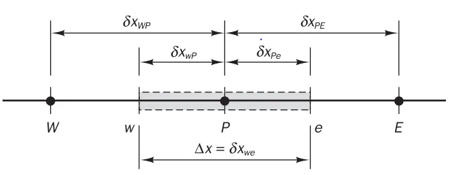
Notation followed, in the furthur analysis

2.Discretisation of equation:

The key step of the finite volume method is the integration of the governing equation (or equations) over a elemental control volume to yield a discretised equation at its nodal point. The volume integrals in the partial differential equations, that contains the divergence term are converted to surface integrals using the divergence theorem. These terms are then evaluated as fluxes at the surfaces of each finite volume. Because the flux entering a given volume is identical to that leaving the adjacent volume, these methods are conservative.

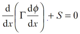
After integration, within the finite control volume, we get

From the above equation, it has the conservation of the property present in it. It is not destroyed in the process of dicretization. A very attractive feature of the finite volume method is that the discretised equation has a clear physical interpretation.

In order to derive useful forms of the discretised equations, the interface diffusion coefficient Γ and the gradient dφ/dx at the boundaries of the elemental control volume are required. To calculate gradients (and hence fluxes) at the control volume faces an approximate distribution of properties between nodal points is used.

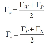
Flux terms are written as follows,

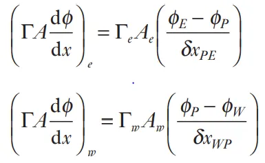
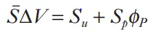
final form of the dicretised equation is as follows

3.Solving the system of algebraic equations:

Discretised equations must be set up at each of the nodal points in order to solve a problem. The resulting system of linear algebraic equations is then solved to obtain the distribution of the property φ at nodal points. Any suitable matrix solution technique may be used for this task.

Major differences between FDM & FVM:

Need for interpolation schemes and flux limiters in FVM:

Interpolation Schemes:

In finite volume methods, evaluation of the terms in the equation (which is obtained after integration of differential equation in the elemental control volume), we require the value of the dependent variable at the surface of the control volume. But we know or solve for the values of the dependent variables, only at the nodal points. So, we need some scheme just like the gradient scheme used in the above formulation for the diffusion term. Interpolation scheme is required for the convective terms of the integrated equation. There are many schemes available for the interpolation.

1. Linear interpolation scheme

2. Upwind interpolation scheme

3. QUICK scheme

4. Hybrid scheme

5. TVD scheme

Flux limiters:

While calculating gradient (in the above example as calculated for diffusion term), some they grow unbouded. These are observed in the shock formations. These high values of gradient will lead to unstable solution. So, we need something to sort this out. Flux limiter comes to our rescue.

Calculating gradients from higher order numerical scheme, will be accurate. But exhibit oscillations near the discontinuities. Where as lower order numerical scheme will be less accurate, stable and numerical diffusion is more at the discontinuities. So to capture shocks accurately, we need to use higher order schemes along with the flux limiters.