Week 3.5 - Deriving 4th order approximation of a 2nd order derivative using Taylor Table method
4th order approximations of the second-order derivative:
We will be using Talor Table Method to formulate the numerical derivative. This method is a convenient and systematic way to deal with, while formulating higher order approximation.
Taylor Table is derived from the Talor series and hence the name. It converts all the bunch of equations into systematic format.
We will be using below pasted Talor table for Numerical scheme formulation.
1. Central Difference Scheme:
The final form of the central difference scheme after formulation is:
`(delta^2(f(i)))/(deltax^2) = af(i-2)+bf(i-1)+cf(i)+df(i+1)+ef(i+2)` here 'i' is used as indexing parameter for 'x' ie, `f(i)=f(x) , f(i+1)=f(x+Deltax)` and so on.
| Taylor's Table terms | ||||||
| Numerical Stencil | f(i) | Δxf'(i) | Δx2f''(i) | Δx3f'''(i) | Δx4f''''(i) | |
| af(i-2) | a | -2a | 4a/2 | -8a/6 | 16a/24 | |
| bf(i-1) | b | -b | b/2 | -b/6 | b/24 | |
| cf(i) | c | 0 | 0 | 0 | 0 | |
| df(i+1) | d | d | d/2 | d/6 | d/24 | |
| ef(i+2) | e | 2e | 4e/2 | 8e/6 | 16e/24 | |
| co-efficients | 0 | 0 | 1 | 0 | 0 | |
writing Talor series expansion for the right hand side terms and taking terms which are common will result in the following equation.
`(delta^2(f(i)))/(deltax^2) = cf(i) + (-2a-b+d+2e)Deltaxf'(i) + (2a+b/2 +d/2+2e)Deltax^2f''(i) +`
`(-(8a)/6-b/6+d/6+(8e)/6)Deltax^3f'''(i)+((16a)/24+b/24+d/24+(16e)/24)Deltax^4f''''(i)+((-32a)/120-b/120+d/120+(32e)/120) ........`
as this is approximately equal to `(del^2(f(i)))/(delx^2)`. Therefore we can write
`(del^2(f(i)))/(delx^2)~~(delta^2(f(i)))/(deltax^2)` and
`(del^2(f(i)))/(delx^2) ~~ (a+b+c+d+e)f(i) + (-2a-b+d+2e)Deltaxf'(i) + (2a+b/2 +d/2+2e)Deltax^2f''(i) +`
`(-(8a)/6-b/6+d/6+(8e)/6)Deltax^3f'''(i)+((16a)/24+b/24+d/24+(16e)/24)Deltax^4f''''(i)+((-32a)/120-b/120+d/120+(32e)/120) ........`
Compaing L.H.S and R.H.S, we get
`(a+b+c+d+e) = 0`
`(-2a-b+d+2e)Deltax = 0`
`(2a+b/2 +d/2+2e)Deltax^2 = 1`
`(-(8a)/6-b/6+d/6+(8e)/6)Deltax^3 = 0`
`((16a)/24+b/24+d/24+(16e)/24)Deltax^4 = 0`
we can solve them by considering suitable `Deltax` value. we get the values for a,b,c,d and e.
2. Skewed right-sided difference or Forward Difference Scheme:
The final form of the forward difference scheme after formulation is:
`(delta^2(f(i)))/(deltax^2) = af(i)+bf(i+1)+cf(i+2)+df(i+3)+ef(i+4)+gf(i+5)`
Using the below mentioned Taylor table, following the similar procedure we get
| Taylor's Table terms | |||||||
| Numerical Stencil | f(i) | Δxf'(i) | Δx2f''(i) | Δx3f'''(i) | Δx4f''''(i) | Δx5f'''''(i) | |
| af(i) | a | 0 | 0 | 0 | 0 | 0 | |
| bf(i+1) | b | b | b/2 | b/6 | b/24 | b/120 | |
| cf(i+2) | c | 2c | 4c/2 | 8c/6 | 16c/24 | 32c/120 | |
| df(i+3) | d | 3d | 9d/2 | 27d/6 | 81d/24 | 243d/120 | |
| ef(i+4) | e | 4e | 16e/2 | 64e/6 | 256e/24 | 1024e/120 | |
| gf(i+5) | g | 5g | 25g/2 | 125g/6 | 625g/24 | 3125g/120 | |
| co-efficients | 0 | 0 | 1 | 0 | 0 | 0 | |
as this is approximately equal to `(del^2(f(i)))/(delx^2)`. Therefore we can write
`(del^2(f(i)))/(delx^2)~~(delta^2(f(i)))/(deltax^2)`
we get following equations,
`a+b+c+d+e+g=0`
`(b+2c+3d+4e+5g)Deltax=0`
`(b/2+2c+(9d)/2+8e+(25g)/2)Deltax^2=1`
`(b/6+(8c)/6+(27d)/6+(62e)/6+(125g)/6)Deltax^3 = 0`
`(b/24+(16c)/24+(81d)/24+(256e)/24+(625g)/24)Deltax^4=0`
`(b/120+(32c)/120+(243d)/120+(1024e)/120+(3125g)/120)Deltax^5=0`
we can solve them by considering suitable `Deltax` value. we get the values for a,b,c,d,e and g.
3. Skewed left-sided difference or Backward Difference Scheme:
The final form of the backward difference scheme after formulation is:
`(delta^2(f(i)))/(deltax^2) = af(i)+bf(i-1)+cf(i-2)+df(i-3)+ef(i-4)+gf(i-5)`
Using the below mentioned Taylor table, following the similar procedure we get
| Taylor's Table terms | |||||||
| Numerical Stencil | f(i) | Δxf'(i) | Δx2f''(i) | Δx3f'''(i) | Δx4f''''(i) | Δx5f'''''(i) | |
| af(i) | a | 0 | 0 | 0 | 0 | 0 | |
| bf(i+1) | b | -b | b/2 | -b/6 | b/24 | -b/120 | |
| cf(i+2) | c | -2c | 4c/2 | -8c/6 | 16c/24 | -32c/120 | |
| df(i+3) | d | -3d | 9d/2 | -27d/6 | 81d/24 | -243d/120 | |
| ef(i+4) | e | -4e | 16e/2 | -64e/6 | 256e/24 | -1024e/120 | |
| gf(i+5) | g | -5g | 25g/2 | -125g/6 | 625g/24 | -3125g/120 | |
| co-efficients | 0 | 0 | 1 | 0 | 0 | 0 | |
as this is approximately equal to `(del^2(f(i)))/(delx^2)`. Therefore we can write
`(del^2(f(i)))/(delx^2)~~(delta^2(f(i)))/(deltax^2)`
we get following equations,
`a+b+c+d+e+g=0`
`(b+2c+3d+4e+5g)Deltax=0`
`(b/2+2c+(9d)/2+8e+(25g)/2)Deltax^2=1`
`(b/6+(8c)/6+(27d)/6+(62e)/6+(125g)/6)Deltax^3 = 0`
`(b/24+(16c)/24+(81d)/24+(256e)/24+(625g)/24)Deltax^4=0`
`(b/120+(32c)/120+(243d)/120+(1024e)/120+(3125g)/120)Deltax^5=0`
We can solve them by considering suitable `Deltax^2` value. we get the values for a,b,c,d and e^2.
Note: Here we need to remember that the a,b,c,d,e and g are different for different schemes.
We will be using Matrix inversion method to calculate co-efficients.
Skewed schemes are fourth-order accurate:
After we evaluate the values a,b,c,d,e and g, they are of the form `(constant)/(Deltax^2)`.
After we calculate the numerical second order derivative, we get
`(delta^2(f(i)))/(deltax^2) = c_1f(i) + (c_2)Deltaxf'(i) + (c_3)Deltax^2f''(i) +`
`(c_4)Deltax^3f'''(i)+(c_5)Deltax^4f''''(i)+(c_6)Deltax^5f'''''(i) ........`
where `c_1,c_2,c_3,c_4,c_5 and c_6` are constant, which are of the form `(constant)/(Deltax)^2`,
we neglect all the terms from (some constants)f''''''(i)`Deltax^4` , so the method is 4th order accurate.
The same can be derived from the Hint-2, we can calculate the same, ie,
The order of accuracy = Number of nodes in the stencil - order of derivative for one-sided/skewed schemes
The order of accuracy = 6-2=4.
We find the second order drivative for the given function using the above derived numerical schemes.
f(x)= `e^x*cos(x)`.
Matlab code for finidng numerical formulations co-efficients, finding derivatives (numerical and analytical) and plotting error graphs for the given function:
In the co-efficients claculation we did not include `Deltax^2`, for simplicity in the code and the dx variable can be declared later in the code .
clc
clear all
close all

% finding the co-efficient for numerical formulation
% in this calculation we are not including dx for simplicity
% we will be using matrix inversion method
%central difference method
A = [1,1,1,1,1;-2,-1,0,1,2;2,0.5,0,0.5,2;-8,-1,0,1,8;16,1,0,1,16];
B=[0;0;1;0;0];
X = (inv(A))*B;
%skewed right sided difference method
A= [1,1,1,1,1,1;0,1,2,3,4,5;0,0.5,2,4.5,8,12.5;0,1,8,27,64,125;0,1,16,81,256,625;0,1,32,243,1024,3125];
B=[0;0;1;0;0;0]
Y = (inv(A))*B;
%skewed left sided difference method
A= [1,1,1,1,1,1;0,1,2,3,4,5;0,0.5,2,4.5,8,12.5;0,1,8,27,64,125;0,1,16,81,256,625;0,1,32,243,1024,3125];
B=[0;0;1;0;0;0]
Z = (inv(A))*B;

% calculating derivatives using numerical and analytical techniques
a = pi/4; % value of x at wich we want to find the derivative
dx = linspace(pi/200,pi/400,40);
% finding the analytical derivative for the given function
syms x
g = exp(x)*cos(x);
diff(g);
diff(ans);
analytical_derivative = ans;
second_derivative_analytical=vpa(subs(analytical_derivative,x,a));
% finding the numerical derivative for the given function
%central difference method
second_derivative_cds = (X(1)*vpa(subs(g,x,a-2*dx))+X(2)*vpa(subs(g,x,a-dx))+X(3)*vpa(subs(g,x,a))+X(4)*vpa(subs(g,x,a+dx))+X(5)*vpa(subs(g,x,a+2*dx)))./dx.^2;
%skewed right sided difference method
second_derivative_fds = (Y(1)*vpa(subs(g,x,a))+Y(2)*vpa(subs(g,x,a+dx))+Y(3)*vpa(subs(g,x,a+2*dx))+Y(4)*vpa(subs(g,x,a+3*dx))+Y(5)*vpa(subs(g,x,a+4*dx))+Y(6)*vpa(subs(g,x,a+5*dx)))./dx.^2;
%skewed left sided difference method
second_derivative_bds = (Z(1)*vpa(subs(g,x,a))+Z(2)*vpa(subs(g,x,a-dx))+Z(3)*vpa(subs(g,x,a-2*dx))+Z(4)*vpa(subs(g,x,a-3*dx))+Z(5)*vpa(subs(g,x,a-4*dx))+Z(6)*vpa(subs(g,x,a-5*dx)))./dx.^2;

% Calculating errors
cds_error = abs(second_derivative_analytical-second_derivative_cds);
fds_error = abs(second_derivative_analytical-second_derivative_fds);
bds_error = abs(second_derivative_analytical-second_derivative_bds);

% plotiing error plots for comparison
figure(1)
plot(dx,cds_error);
hold on
plot(dx,fds_error);
plot(dx,bds_error);
grid on
title('plot comparing the absolute error between cds, fds and bds at x=pi/4')
xlabel('dx')
ylabel('error')
legend('central difference scheme', 'forward difference scheme','backward difference scheme')

figure(2)
loglog(dx,cds_error);
hold on
loglog(dx,fds_error);
loglog(dx,bds_error);
grid on
title('plot comparing the absolute error between cds, fds and bds at x=pi/4')
xlabel('log(dx)')
ylabel('log(error)')
legend('central difference scheme', 'forward difference scheme','backward difference scheme')
Results:
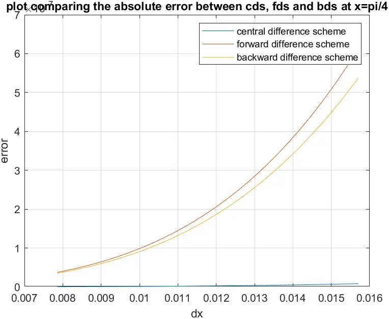
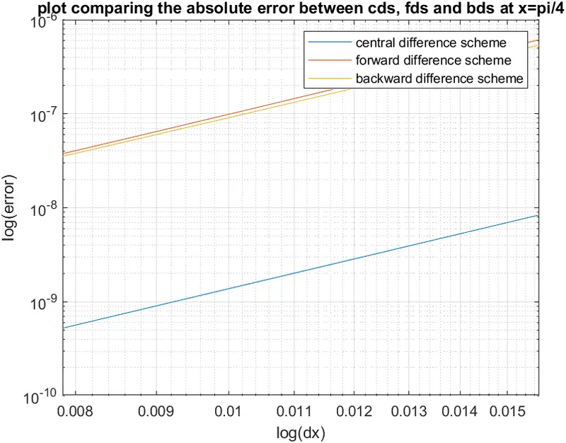
Remarks:
1. We can notice from the second plot, the slopes of the curves are the same. This is beacause all the numerical scemes are fourth order approximate.
2. From the first plot, both the forward and backward difference formula gives the same error approximately (This need not be true all the time, as it depends on step size).
3. Central difference formula is giving better results. (This need not be true all the time, as it depends on the step size dx).
What can a skewed scheme do that a CD scheme cannot?
When we discretise a governing differential equation or derive a numerical scheme to solve a problem, generally it will be applicable to the entire domain in which the governing equation is valid. It means we can apply the dicretised equation at each and every grid point. When it comes to boundary of the domain, central difference scheme cannot be used as the grid points are available only on one side. In such conditions, skewed schemes are applied. On the right boundary, we use left skewed scheme. And on the left boundary, we use right skewed scheme.