Week 5.1 - Mid term project - Solving the steady and unsteady 2D heat conduction problem
Aim:
Solving 2D heat conduction equation by Steady state analysis & Transient State Analysis by implicit and explicit method using iterative techniques like Jacobi, Gauss Seidel and SOR method.
Inputs:
Domain: square slab (1m x 1m)
Top Boundary condition= 600 K
Bottom Boundary condition = 900 K
Left Boundary condition = 400 K
Right Boundary condition = 800 K
Boundary condition at the corner of the domain will become the arithmetic mean of boundary conditions of the edges forming the corner.
Your absolute error criteria or tolerance is 1e-4
Number of grid points in x and y direction are same and equal to 10 (nx = ny = 10)
Relaxation factor for SOR is 1.04
Thermal diffisivity =1.5
Classification of the ways by which we are going to solve the problem:
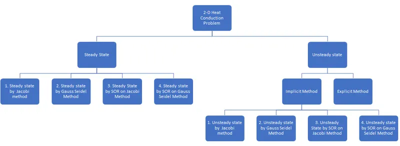
We will be writing three Matlab codes
a) Steady state (All the four iterative methods)
b) Unsteady Implicit (All the four iterative methods)
c) Unsteady Explict Method
Governing Differential Equation and Notation:
The governing differential equation which govern the 2-D Heat Conduction is given by
`(delT)/(delt) = alpha((del^2T)/(delx^2) + (del^2T)/(dely^2))` where `alpha` is thermal diffisivity.
We will be using different numerical schemes to discretize the equation and Matlab code will be written after each discretization to get the solution of the problem and final solution plots will be pasted. And then we will proceed for the next method.
Notation we will be following during descretization is as follows:
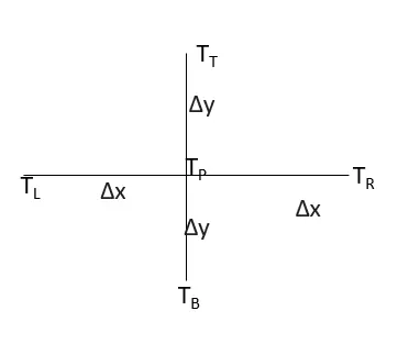
Where P is current node, L is the left node, R is the right node, T is the top node and B is the bottom node.
a) Steady state:
The governing differential equation for the steady state heat conduction is
`(del^2T)/(delx^2) + (del^2T)/(dely^2) = 0`
Upon discretizing this eqaution using central difference scheme, we get
`(T_L - 2T_P + T_R)/(Deltax^2) + (T_T - 2T_P + T_B)/(Deltay^2)=0`
on simplification, we get
`T_P = 1/k*((T_L + T_R)/(Deltax^2) + (T_B + T_T)/(Deltay^2))`
where `k = (2(Deltax^2 + Deltay^2))/(Deltax^2Deltay^2)`
Now by using the above dicretized equation and the input information, we will be writing the Matlab code to solve the problem using all the iterative method.
Matlab code:
% this code will solve the 2D steady state heat conduction problem using
% the four iteratve techniques
close all
clear all
clc


%input variables
L = 1; %length of the slab or domain
H =1; % height of slab or domain
nx =10; %no of grid points in the length direction
ny =10; %no of grid points in y direction
tolerance= 1e-4; % error should be less that tolerance for stopping the iteration
alpha = 1.5; % thermal diffisivty

w = 1.04; % relaxation factor
x = linspace(0,L,nx);
y = linspace(0,H,ny);
iteration_method = [1 2 3 4 ] ;% Changing this we can choose different iterative svhemes
%1 -jacobi
%2 - gauss seidel method
%3 - sor over jacobi
%4 - sor over gauss seidel
T_t=600;
T_b=900;
T_l = 400;
T_r = 800;

%step sizes calculation
dx = L/(nx-1);
dy=H/(ny-1);


% declaring the variable which store the temperature and inputing initial
% and boundary conditions
T = ones(ny,nx); %initialising variable
T = 300*T; %initial condition

% boundary conditions
T(1,:) = T_t;
T(ny,:) = T_b;
T(:,1) = T_l;
T(:,nx) = T_r;

%declaring edge temperature
T(1,1)=(T_l+T_t)/2;
T(ny,1)=(T_l+T_b)/2;
T(1,nx)=(T_t+T_r)/2;
T(ny,nx)=(T_r+T_b)/2;

% creating initial temperature variable
T_initial = T;
T_old = T_initial;
%variable of convnience
k = 2*(dx^2 + dy^2)/(dx^2*dy^2);


%index
%m is for iteratin method
%i is for nodes along y direction
%j is for nodes along x direction


for m = 1:length(iteration_method)
    T = T_initial;
    T_old=T_initial;
    error = 1000;
    iteration = 0;
    while error> tolerance
        for i = 2:ny-1
            for j=2:nx-1
                if m==1
                    T(i,j) = ((T_old(i,j-1)+T_old(i,j+1))/(k*dx^2)) + ((T_old(i-1,j)+T_old(i+1,j))/(k*dy^2));
                end
                if m ==2
                    T(i,j) = ((T(i,j-1)+T(i,j+1))/(k*dx^2)) + ((T(i-1,j)+T(i+1,j))/(k*dy^2));
                end
                if m==3
                    T_ja = ((T_old(i,j-1)+T_old(i,j+1))/(k*dx^2)) + ((T_old(i-1,j)+T_old(i+1,j))/(k*dy^2));
                    T(i,j) = T_old(i,j) + w*(T_ja-T_old(i,j));

                end
                if m==4
                    T_gs = ((T(i,j-1)+T(i,j+1))/(k*dx^2)) + ((T(i-1,j)+T(i+1,j))/(k*dy^2));
                    T(i,j) = T_old(i,j) + w*(T_gs-T_old(i,j));
                end
            end
        end
        error = max(max(abs(T_old-T)));
        T_old=T;
        iteration =iteration+1;
    end
    % plotting
    figure(m)
    contourf(x,y,T)
    clabel(contourf(x,y,T))
    set(gca,'ydir','reverse')
    colorbar
    colormap(jet)
    if m==1
        title( sprintf('Jacobi Method (number of iterations = %d)',iteration))
    end
    if m==2
        title( sprintf('Gauss Seidel Method (number of iterations = %d)',iteration))
    end
    if m==3
        title( sprintf('SOR over Jacobi Method (number of iterations = %d)',iteration))
    end
    if m==4
        title( sprintf('SOR over Gauss Seidel Method (number of iterations = %d)',iteration))
    end
end
Plots:
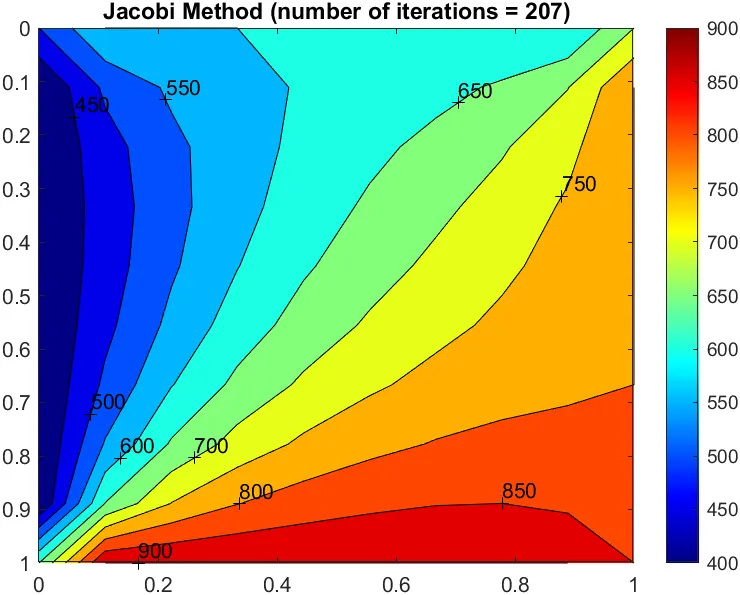
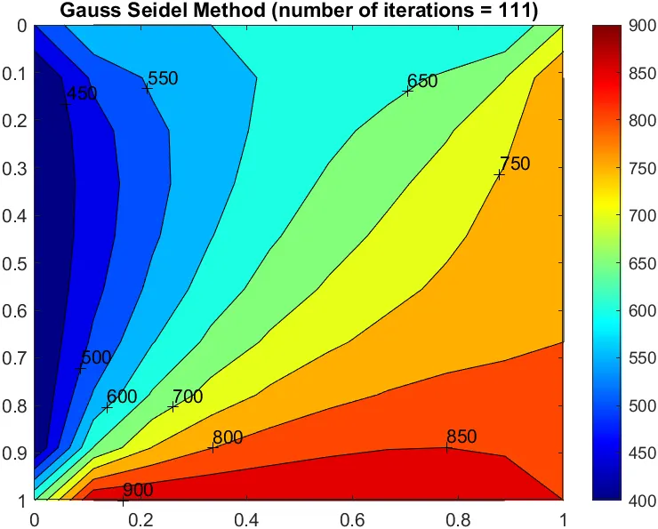
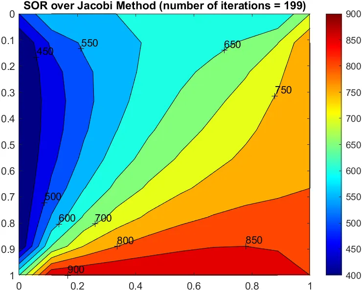
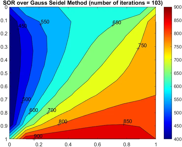
In the above plots relaxation factor of w=1.04 is used, because for larger value for SOR over Jacobi method solution was going unstable.
b) Unsteady Implicit Method:
The governing differential equation for the steady state heat conduction is
`(delT)/(delt)=alpha((del^2T)/(delx^2) + (del^2T)/(dely^2) )`
Upon discretizing this eqaution using central difference scheme for space derivative and forward differencing scheme for time derivative, we get
`(T_p(n+1)-T_P(n))/(Deltat)=alpha((T_L - 2T_P + T_R)/(Deltax^2) + (T_T - 2T_P + T_B)/(Deltay^2))`
RHS evaluated at 'n+1' time step
here 'n' corresponds to time index
on simplification, we get
`T_P(n+1) = (T_p(n)+k_1(T_L(n+1)+T_R(n+1))+k_2(T_T(n+1)+T_B(n+1)))/k`
where `k_1 = (alpha*DeltaT)/(Deltax^2)`,`k_2 = (alpha*DeltaT)/(Deltay^2)` and `k = 1+2k_1+2k_2`
Now by using the above dicretized equation and the input information, we will be writing the Matlab code to solve the problem using all the iterative method.
Matlab code:
% this code will solve the 2D unsteady state heat conduction problem by implicit with time using
% the four iteratve techniques
close all
clear all
clc


%input variables
L = 1; %length of the slab or domain
H =1; % height of slab or domain
nx =10; %no of grid points in the length direction
ny =10; %no of grid points in y direction
tolerance= 1e-4; % error should be less that tolerance for stopping the iteration
alpha = 1.5; % thermal diffisivty

w = 1.04; % relaxation factor
x = linspace(0,L,nx);
y = linspace(0,H,ny);
iteration_method = [1 2 3 4 ] ;% Changing this we can choose different iterative svhemes
%1 -jacobi
%2 - gauss seidel method
%3 - sor over jacobi
%4 - sor over gauss seidel
T_t=600;
T_b=900;
T_l = 400;
T_r = 800;

%step sizes calculation
dx = L/(nx-1);
dy=H/(ny-1);
dt = 0.001; % time step calculated based on CFL number criterion


% declaring the variable which store the temperature and inputing initial
% and boundary conditions
T = ones(ny,nx); %initialising variable
T = 300*T; %initial condition

% boundary conditions
T(1,:) = T_t;
T(ny,:) = T_b;
T(:,1) = T_l;
T(:,nx) = T_r;

%declaring edge temperature
T(1,1)=(T_l+T_t)/2;
T(ny,1)=(T_l+T_b)/2;
T(1,nx)=(T_t+T_r)/2;
T(ny,nx)=(T_r+T_b)/2;

% creating initial temperature variable
T_initial = T;
T_old = T_initial;
%variable of convnience
k1 = (alpha*dt)/dx^2;
k2 = (alpha*dt)/dy^2;
k = 1 + 2*k1 + 2*k2;


%index
%m is for iteratin method
%n is for index along time
%i is for nodes along y direction
%j is for nodes along x direction


for m = 1:length(iteration_method)
    T = T_initial;
    T_old=T_initial;
    T_prev = T_initial;
    error = 1000;
    iteration = 0;
    while error > tolerance % time loop
        while error> tolerance %space loop
            for i = 2:ny-1
                for j=2:nx-1
                    if m==1
                        T(i,j) = (T_prev(i,j) + k1*(T_old(i,j-1)+T_old(i,j+1))+ k2*(T_old(i-1,j)+T_old(i+1,j)))/k;
                    end
                    if m ==2
                         T(i,j) = (T_prev(i,j) + k1*(T(i,j-1)+T(i,j+1))+ k2*(T(i-1,j)+T(i+1,j)))/k;
                    end
                    if m==3
                         T_ja = (T_prev(i,j) + k1*(T_old(i,j-1)+T_old(i,j+1))+ k2*(T_old(i-1,j)+T_old(i+1,j)))/k;
                        T(i,j) = T_old(i,j) + w*(T_ja-T_old(i,j));

                    end
                    if m==4
                        T_gs = (T_prev(i,j) + k1*(T(i,j-1)+T(i,j+1))+ k2*(T(i-1,j)+T(i+1,j)))/k;
                        T(i,j) = T_old(i,j) + w*(T_gs-T_old(i,j));
                    end
                end
            end
            error = max(max(abs(T_old-T)));
            T_old=T;
            iteration =iteration+1;
        end
        error =  max(max(abs(T_prev-T)));

        T_prev = T;
    end
    % plotting
    figure(m)
    contourf(x,y,T)
    clabel(contourf(x,y,T))
    set(gca,'ydir','reverse')
    colorbar
    colormap(jet)
    if m==1
        title( sprintf('Jacobi Method (total iterations for steady state= %d)',iteration))
    end
    if m==2
        title( sprintf('Gauss Seidel Method (total iterations for steady state= %d)',iteration))
    end
    if m==3
        title( sprintf('SOR over Jacobi Method (total iterations for steady state= %d)',iteration))
    end
    if m==4
        title( sprintf('SOR over Gauss Seidel Method (total iterations for steady state= %d)',iteration))
    end
end
Plots:
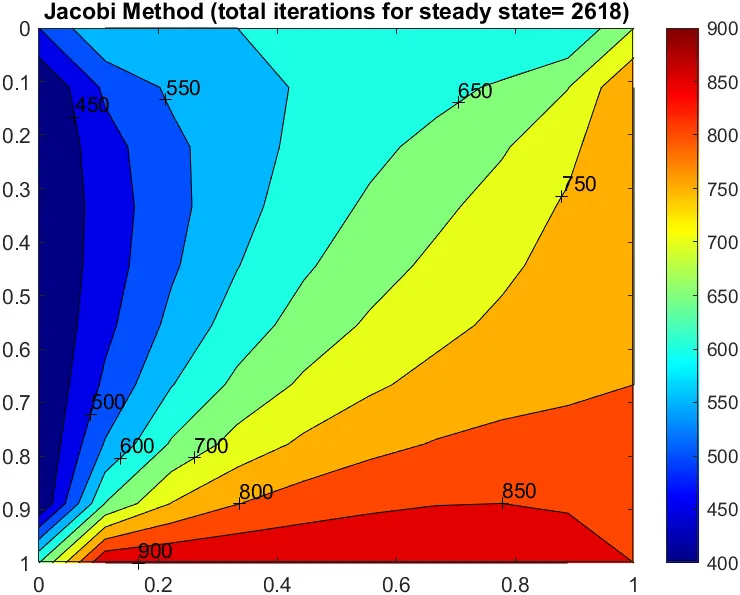
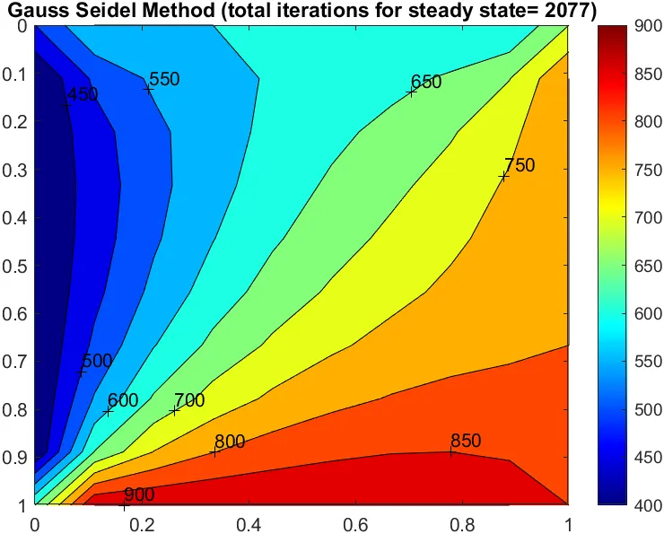
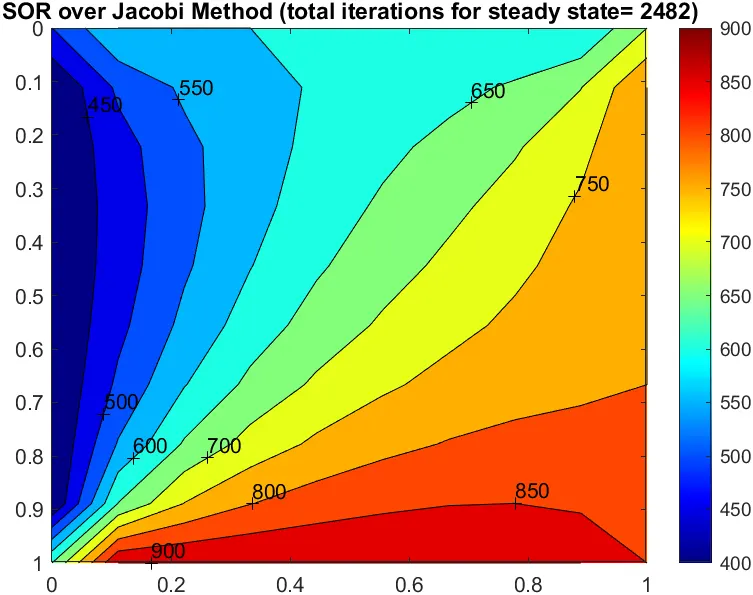
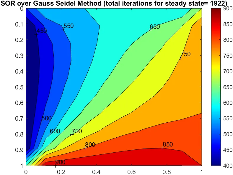
Number of iterations specified in the plots are space iterations multiplied by time iterations. And relaxation factor is 1.04 and time step is 0.001.
c) Unsteady Explict Method:
The governing differential equation for the steady state heat conduction is
`(delT)/(delt)=alpha((del^2T)/(delx^2) + (del^2T)/(dely^2) )`
Upon discretizing this eqaution using central difference scheme and forward differencing scheme for time derivative, we get
`(T_p(n+1)-T_P(n))/(Deltat)=alpha((T_L - 2T_P + T_R)/(Deltax^2) + (T_T - 2T_P + T_B)/(Deltay^2))`
RHS evaluated at 'n' time step
here 'n' corresponds to time index
on simplification, we get
`T_P(n+1) = ((1-2k_1-2k_2)T_P(n)+k_1(T_L(n)+T_R(n))+k_2(T_T(n)+T_B(n)))`
where `k_1 = (alpha*DeltaT)/(Deltax^2)`,`k_2 = (alpha*DeltaT)/(Deltay^2)`
Now by using the above dicretized equation and the input information, we will be writing the Matlab code to solve the problem.
Matlab code:
% this code will solve the 2D unsteady state heat conduction problem by explicit with time

close all
clear all
clc


%input variables
L = 1; %length of the slab or domain
H =1; % height of slab or domain
nx =10; %no of grid points in the length direction
ny =10; %no of grid points in y direction
tolerance= 1e-4; % error should be less that tolerance for stopping the iteration
alpha = 1.5; % thermal diffisivty


x = linspace(0,L,nx);
y = linspace(0,H,ny);
T_t=600;
T_b=900;
T_l = 400;
T_r = 800;

%step sizes calculation
dx = L/(nx-1);
dy=H/(ny-1);
dt = 0.001; % time step calculated based on CFL number criterion


% declaring the variable which store the temperature and inputing initial
% and boundary conditions
T = ones(ny,nx); %initialising variable
T = 300*T; %initial condition

% boundary conditions
T(1,:) = T_t;
T(ny,:) = T_b;
T(:,1) = T_l;
T(:,nx) = T_r;

%declaring edge temperature
T(1,1)=(T_l+T_t)/2;
T(ny,1)=(T_l+T_b)/2;
T(1,nx)=(T_t+T_r)/2;
T(ny,nx)=(T_r+T_b)/2;

% creating initial temperature variable
T_initial = T;
T_prev = T_initial;
%variable of convnience
k1 = (alpha*dt)/dx^2;
k2 = (alpha*dt)/dy^2;
k = 1 - 2*k1 - 2*k2;

%index
%n is for index along time
%i is for nodes along y direction
%j is for nodes along x direction
error =100;
iteration=0;
while error > tolerance
    for i = 2:ny-1
        for j=2:nx-1
            T(i,j)= k*T_prev(i,j) + k1*(T_prev(i,j-1)+T_prev(i,j+1)) + k2*(T_prev(i-1,j)+T_prev(i+1,j));
        end
    end
    iteration = iteration+1;
    error =  max(max(abs(T_prev-T)));
    T_prev = T;
end
% plotting
figure(1)
contourf(x,y,T)
clabel(contourf(x,y,T))
set(gca,'ydir','reverse')
colorbar
colormap(jet)
title( sprintf('Unsteady Explicit (total iterations for steady state= %d)',iteration))
Plots:
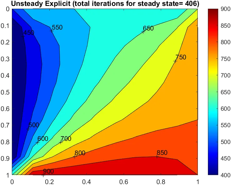
Remarks:
1. Number of iterations: Jacobi method > Gauss Seidel method > SOR method.
2. When we are solving for steady state conditions, it is better to use Steady state analysis. And thereby we can reduce the number of iterations alot.
3.Applying SOR on Jacobi and Gauss Seidel method, helps in converging faster.
| 2-D Heat Conduction Problem | Method | No of iterations |
| Steady State | Jacobi method | 207 |
| Gauss Seidel Method | 111 | |
| SOR on Jacobi Method | 199 | |
| SOR on Gauss Seidel Method | 103 | |
| Unsteady Implicit | Jacobi method | 2618 |
| Gauss Seidel Method | 2077 | |
| SOR on Jacobi Method | 2482 | |
| SOR on Gauss Seidel Method | 1922 | |
| Unsteady Explicit | 406 |