Week 7 - Simulation of a 1D Super-sonic nozzle flow simulation using Macormack Method
Simulation of a 1D Super-sonic nozzle flow using Macormack Method:
In this exercise, we are going to simulate the isentropic flow through a quasi 1D subsonic-supersonic nozzle using Macormack Method. We will be using both the conservation and non-conservation forms of the equations. We will be doing the following things in this report:
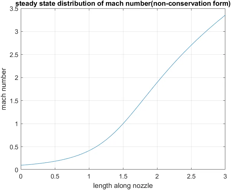
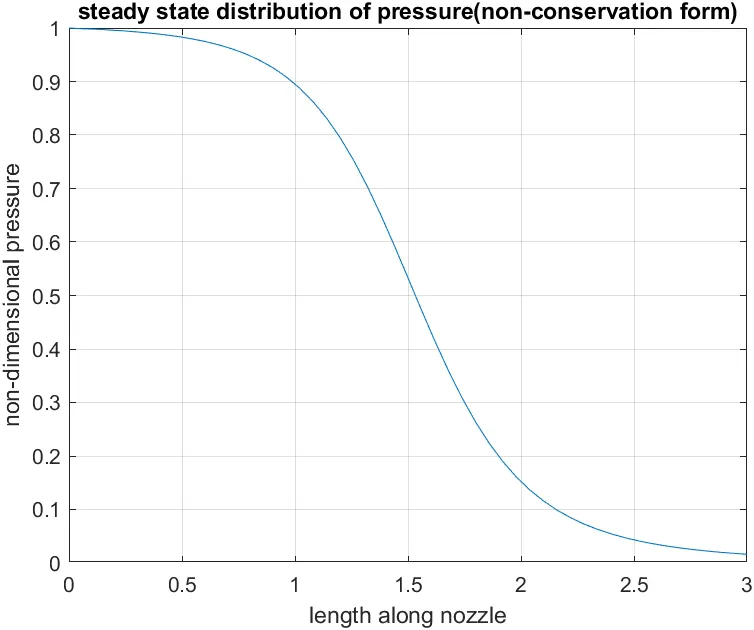
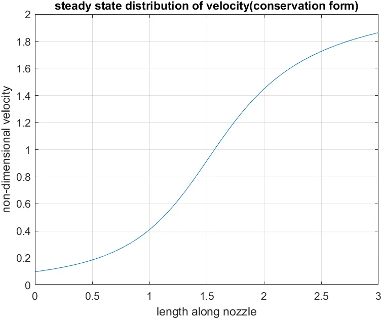
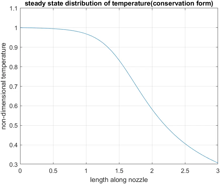
1. Steady-state distribution of primitive variables inside the nozzle
2. Time-wise variation of the primitive variables
3. Variation of Mass flow rate distribution inside the nozzle at different time steps during the time-marching process
4. Comparison of Normalized mass flow rate distributions of both forms
5. Perform grid independence test for both the methods.
By doing so, we will compare the results from conservation form method and non-conservation form method.
Conservation and non-conservation forms of the governing equations:
We will be writing the final form of the governing equations which are used for writing computer program for both conservation and non-conservation forms.
These equation are obtained by applying the integral form of the governing equations to the elemental length of the nozzle. Upon simplification, we get both conservation and non-conservation forms. These two different forms are one and the same and we can get one form by starting with other form. They are analytically one and the same. But when we solve them numerically, different forms of the equations give different solution. Conservation form provides the advantage of easy understanding and implementing in the computer program. It also give good results, when there are discontinuities in the domain. However, there are applications of both these forms. The equation which we will be writing below are in non-dimensional form. These equations are non-dimensionalised using the stagnation temperature, length of nozzle, stagnation pressure, stagnation density, throat area and sonic velocity at stagnation condition.
Non - conservation form:
Continuity equation:

Momentum equation:
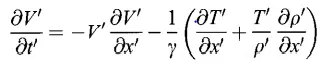
Energy equation:

In getting to these equations, we used equation of state.
Conservation form:
Continuity equation:
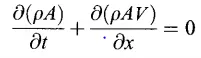
Momentum equation:

Energy equation:

we will be using following equation for discretization, in getting numerical solution.
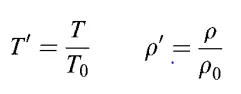
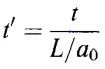
Non-dimensional quantities are defined in the following manner:



The numerical method used is Macormack Method. It is a two step explicit time marching method. Here two step indicates, predictor and corrector step. Predictor step is forward differencing and Corrector step is backward differencing. The advantage of this method is, we get second order accurate numerical scheme without evaluating second order derivative in the solution. This is a simplification for the Lax-Wendroff method, but not compromising on accuracy of the solution.
For calculating time step, we used the stability criterion at each and every point, the smallest of the time step at all the nodes is used for programming. The time step is calculated using the expression:
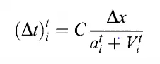
where 'C' is Courant number, 'a' is sonic velocity, 'v' is actual velocity and 'dx' is distance between two nodes.
The above expression is derived for a linear differential equation, but we can use it for non-linear equation satisfactorily. So, we take safe value of 'C' as 0.5.
Matlab Code:
Following Matlab code is used for getting results and plots.
% main script for gettting plots. we will be using the function to run
% consevation and non-conservation form
clear all
close all
clc

% inputs
n = 101; % number of nodes along x
x = linspace(0,3,n);%  nodes along 'x'
dx = x(2) - x(1); % step size along x_ direction
g = 1.4; % specific heat ratio


% initial conditions
rho = 1 - 0.3146*x; % r is denoting density
t = 1-0.2314*x;% is denoting temperature
v = (0.1+1.09*x).*t.^(0.5);
c = t.^(0.5); %sonic velocity in the medium


%area profile
a = 1 + 2.2*(x-1.5).^2;

% we will be using the time steps calculated from stability criterion
nt = 2000; % number of time steps
C = 0.5;  % CFL number is taken here
%getting solution for non_conservation form (we use subscript of 1)
[velocity1 , density1, temperature1, sonic_velocity1, time1] = non_conservative_form(n,dx,g,rho,t,v,c,a,nt,C);
%getting solution for the conservation form (we use subscript 2)
[velocity2 , density2, temperature2, sonic_velocity2, time2] = conservative_form(n,dx,g,rho,t,v,c,a,nt,C);

figure(1)
plot(x,velocity1(nt,:));
grid on
title('steady state distribution of velocity(non-conservation form)')
xlabel('length along nozzle')
ylabel('non-dimensional velocity')


figure(2)
plot(x,temperature1(nt,:));
grid on
title('steady state distribution of temperature(non-conservation form)')
xlabel('length along nozzle')
ylabel('non-dimensional temperature')


figure(3)
plot(x,density1(nt,:));
grid on
title('steady state distribution of density(non-conservation form)')
xlabel('length along nozzle')
ylabel('non-dimensional density')


figure(4)
plot(x,velocity1(nt,:)./sonic_velocity1(nt,:));
grid on
title('steady state distribution of mach number(non-conservation form)')
xlabel('length along nozzle')
ylabel('mach number')

figure(5)
plot(x,density1(nt,:).*temperature1(nt,:));
grid on
title('steady state distribution of pressure(non-conservation form)')
xlabel('length along nozzle')
ylabel('non-dimensional pressure')


figure(6)
plot(x,velocity2(nt,:));
grid on
title('steady state distribution of velocity(conservation form)')
xlabel('length along nozzle')
ylabel('non-dimensional velocity')


figure(7)
plot(x,temperature2(nt,:));
grid on
title('steady state distribution of temperature(conservation form)')
xlabel('length along nozzle')
ylabel('non-dimensional temperature')


figure(8)
plot(x,density2(nt,:));
grid on
title('steady state distribution of density(conservation form)')
xlabel('length along nozzle')
ylabel('non-dimensional density')


figure(9)
plot(x,velocity2(nt,:)./sonic_velocity2(nt,:));
grid on
title('steady state distribution of mach number(conservation form)')
xlabel('length along nozzle')
ylabel('mach number')

figure(10)
plot(x,density2(nt,:).*temperature2(nt,:));
grid on
title('steady state distribution of pressure(conservation form)')
xlabel('length along nozzle')
ylabel('non-dimensional pressure')
% calculating node of the throat
h = round((n+1)/2);
% plotting of variation of variables with time at throat for non-conservation
% form

figure(11)
subplot(5,1,1)
plot(time1, velocity1(:,h))
grid on
title('variation of non dimensional variables with time at throat(non-conservation form))')
ylabel('velocity')

subplot(5,1,2)
plot(time1, temperature1(:,h))
grid on
ylabel('temperature')

subplot(5,1,3)
plot(time1, density1(:,h))
grid on
ylabel('density')

subplot(5,1,4)
plot(time1, velocity1(:,h)./sonic_velocity1(:,h))
grid on
ylabel('Mach number')

subplot(5,1,5)
plot(time1, density1(:,h).*temperature1(:,h))
grid on
xlabel('time in sec')
ylabel('pressure')
% plotting of variation of variables with time at throat for conservation
% form
figure(12)
subplot(5,1,1)
plot(time2, velocity2(:,h))
grid on
title('variation of non dimensional variables with time at throat(conservation form))')
ylabel('velocity')

subplot(5,1,2)
plot(time2, temperature2(:,h))
grid on
ylabel('temperature')

subplot(5,1,3)
plot(time2, density2(:,h))
grid on
ylabel('density')

subplot(5,1,4)
plot(time2, velocity2(:,h)./sonic_velocity2(:,h))
grid on
ylabel('Mach number')

subplot(5,1,5)
plot(time2, density2(:,h).*temperature2(:,h))
grid on
xlabel('time in sec')
ylabel('pressure')
%Variation of Mass flow rate distribution inside the nozzle at different
%time steps during the time-marching process for non-conservation form
figure(13)
plot(x,density1(round(nt/4),:).*a.*velocity1(round(nt/4),:))
grid on
hold on
plot(x,density1(round(nt/3.5),:).*a.*velocity1(round(nt/3.5),:))
plot(x,density1(round(nt/3),:).*a.*velocity1(round(nt/3),:))
plot(x,density1(round(nt/2.5),:).*a.*velocity1(round(nt/2.5),:))
plot(x,density1(round(nt),:).*a.*velocity1(round(nt),:))
legend(sprintf('%d  time step',round(nt/4)),sprintf('%d  time step',round(nt/3.5)),sprintf('%d  time step',round(nt/3)),sprintf('%d  time step',round(nt/2.5)),sprintf('%d  time step',round(nt)))
xlabel('length along the nozzle')
ylabel('non-dimensional mass flow rate')
title('non-dimensional mass flow rate distribution for non-conservation form')
%Variation of Mass flow rate distribution inside the nozzle at different
%time steps during the time-marching process for conservation form
figure(14)
plot(x,density2(round(nt/4),:).*a.*velocity2(round(nt/4),:))
grid on
hold on
plot(x,density2(round(nt/3.5),:).*a.*velocity2(round(nt/3.5),:))
plot(x,density2(round(nt/3),:).*a.*velocity2(round(nt/3),:))
plot(x,density2(round(nt/2.5),:).*a.*velocity2(round(nt/2.5),:))
plot(x,density2(round(nt),:).*a.*velocity2(round(nt),:))
legend(sprintf('%d  time step',round(nt/4)),sprintf('%d  time step',round(nt/3.5)),sprintf('%d  time step',round(nt/3)),sprintf('%d  time step',round(nt/2.5)),sprintf('%d  time step',round(nt)))
xlabel('length along the nozzle')
ylabel('non-dimensional mass flow rate')
title('non-dimensional mass flow rate distribution for conservation form')
% plot to compare ateady atate mass flow rate distribution for
% non-conservation and conservation form
figure(15)

plot(x,density1(nt,:).*a.*velocity1(nt,:))
hold on
grid on
plot(x,density2(nt,:).*a.*velocity2(nt,:))
xlabel('length along the nozzle')
ylabel('non-dimensional mass flow rate')
title('non-dimensional mass flow rate comparison for non-conservation and conservation form')
legend('Non-conservation form','Conservation form')
Function code used for non-conservation form method:
% function for non-conservation form
function [velocity , density, temperature, sonic_velocity, time] = non_conservative_form(n,dx,g,rho,t,v,c,a,nt,C)
time = zeros(1,nt);% stores time data
time(1) = 0; %initial time
m = 0;% variable for convenience for storing time
% we will bw defining defining two dimensional variables to propeeties at
% each time step
density  = zeros(nt,n);
temperature  = zeros(nt,n);
velocity  = zeros(nt,n);
sonic_velocity = zeros(nt,n);

density(1,:)= rho;
velocity(1,:) = v;
temperature(1,:) = t;
sonic_velocity(1,:) = c;

% outer time loop
for k = 1:nt
    dt = min((C*dx)./(v+c));

    rho_old = rho;
    v_old = v;
    t_old = t;

    % predictor method

    for j= 2:n-1
    dvdx = (v(j+1)-v(j))/dx;
    drhodx = (rho(j+1)-rho(j))/dx;
    dtdx = (t(j+1)-t(j))/dx;
    dlogadx = (log(a(j+1))-log(a(j)))/dx;

    % continuity equation
    drhodt_p(j) = -rho(j)*dvdx -rho(j)*v((j))*dlogadx -v(j)*drhodx;

    % momentum equation
    dvdt_p(j) = -v(j)*dvdx -(1/g)*(dtdx + (t(j)/rho(j))*drhodx);

    %energy equation
    dtdt_p(j) = -v(j)*dtdx -(g-1)*t(j)*(dvdx + v(j)*dlogadx);


    end

    %solution update
    for j = 2:n-1
     v(j) = v(j) + dvdt_p(j)*dt;
     rho(j) = rho(j) + drhodt_p(j)*dt;
     t(j) = t(j) + dtdt_p(j)*dt;
    end

    % corrector method
    for j= 2:n-1
    dvdx = (v(j)-v(j-1))/dx;
    drhodx = (rho(j)-rho(j-1))/dx;
    dtdx = (t(j)-t(j-1))/dx;
    dlogadx = (log(a(j))-log(a(j-1)))/dx;

    % continuity equation
    drhodt_c(j) = -rho(j)*dvdx -rho(j)*(v(j))*dlogadx -v(j)*drhodx;

    % momentum equation
    dvdt_c(j) = -v(j)*dvdx -(1/g)*(dtdx + (t(j)/rho(j))*drhodx);

    %energy equation
    dtdt_c(j) = -v(j)*dtdx -(g-1)*t(j)*(dvdx + v(j)*dlogadx);


    end
    for j=2:n-1
     v(j) = v_old(j) + 0.5*(dvdt_p(j)+dvdt_c(j))*dt;
     rho(j) = rho_old(j) + 0.5*(drhodt_p(j)+ drhodt_c(j))*dt;
     t(j) = t_old(j) + 0.5*(dtdt_p(j) + dtdt_c(j))*dt;
    end
     % apply the boundary conditions
     %inlet
     v(1)=2*v(2)-v(3);

     %outlet
     v(n) = 2*v(n-1)-v(n-2);
     rho(n) = 2*rho(n-1)-rho(n-2);
     t(n) = 2*t(n-1)-t(n-2);
     c  = t.^(0.5);

     velocity(k+1,:) =v;
     density(k+1,:) = rho;
     temperature(k+1,:) = t;
     sonic_velocity(k+1,:) = c;
     m = dt+m;
     time(k+1) = m;


    end
Function code used for conservation form method:
% function for conservation form
function [velocity , density, temperature, sonic_velocity, time] = conservative_form(n,dx,g,rho,t,v,c,a,nt,C)
time = zeros(1,nt);% stores time data
time(1) = 0; %initial time
m = 0;% variable for convenience for storing time
% we will bw defining defining two dimensional variables to propeeties at
% each time step
density  = zeros(nt,n);
temperature  = zeros(nt,n);
velocity  = zeros(nt,n);
sonic_velocity = zeros(nt,n);

density(1,:)= rho;
velocity(1,:) = v;
temperature(1,:) = t;
sonic_velocity(1,:) = c;

% initial conditions
U1 = rho.*a;
U2 = U1.*v;
U3 = rho.*(t/(g-1) + (g/2)*(v.^2)).*a;


% outer time loop
for k = 1:nt

    dt = min((C*dx)./(v+c));

    U1_old = U1;
    U2_old = U2;
    U3_old = U3;

    F1 = U2;
    F2 = (U2.^2./U1) + ((g-1)/g)*(U3 - ((g/2)*(U2.^2./U1)));
    F3 = (g.*U2.*U3)./U1 - (g*(g-1)/2)*(U2.^3./U1.^2);
    J = ((g-1)/g)*(U3 - (g/2)*(U2.^2./U1));


    % predictor method
    for j= 2:n-1


        % continuity equation
        dU1dt_p(j) = -(F1(j+1)-F1(j))/dx;

        % momentum equation
        dU2dt_p(j) = -(F2(j+1)-F2(j))/dx + J(j)*(log(a(j+1))-log(a(j)))/dx ;

        %energy equation
        dU3dt_p(j) =  -(F3(j+1)-F3(j))/dx;

    end

    %solution update
    for j=2:n-1
       U1(j) = U1(j) +  dU1dt_p(j)*dt;
       U2(j) = U2(j) +  dU2dt_p(j)*dt;
       U3(j) = U3(j) +  dU3dt_p(j)*dt;

    end


    %corrector method
    F1 = U2;
    F2 = (U2.^2./U1) + ((g-1)/g)*(U3 - ((g/2)*(U2.^2./U1)));
    F3 = (g.*U2.*U3)./U1 - (g*(g-1)/2)*(U2.^3./U1.^2);
    J = ((g-1)/g)*(U3 - (g/2)*(U2.^2./U1));

    for j= 2:n-1


        % continuity equation
        dU1dt_c(j) = -(F1(j)-F1(j-1))/dx;

        % momentum equation
        dU2dt_c(j) = -(F2(j)-F2(j-1))/dx + J(j)*(log(a(j))-log(a(j-1)))/dx;

        %energy equation
        dU3dt_c(j) =  -(F3(j)-F3(j-1))/dx;


    end
    for j=2:n-1
        U1(j) = U1_old(j) + 0.5*(dU1dt_p(j)+dU1dt_c(j))*dt;
        U2(j) = U2_old(j) + 0.5*(dU2dt_p(j)+ dU2dt_c(j))*dt;
        U3(j) = U3_old(j) + 0.5*(dU3dt_p(j) + dU3dt_c(j))*dt;
    end
     % apply the boundary conditions
     %inlet
     U2(1) = 2*U2(2) - U2(3);
     U3(1) = U1(1)*(t(1)/(g-1) + (g/2)*(U2(1)/U1(1))^2);

     %outlet
     U1(n) = 2*U1(n-1) - U1(n-2);
     U2(n) = 2*U2(n-1) - U2(n-2);
     U3(n) = 2*U3(n-1) - U3(n-2);
     rho = U1./a;
     v = U2./U1;
     t = (g-1)*(U3./U1 - (g/2)*(U2./U1).^2);
     p = rho.*t;
     c = t.^(0.5);

     velocity(k+1,:) =v;
     density(k+1,:) = rho;
     temperature(k+1,:) = t;
     sonic_velocity(k+1,:) = c;
     m = dt+m;
     time(k+1) = m;


    end
Plots:
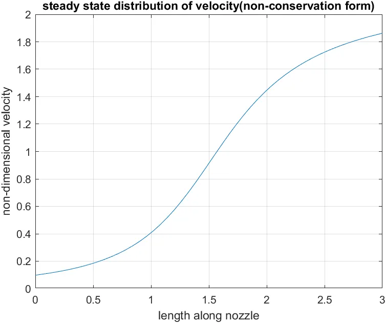
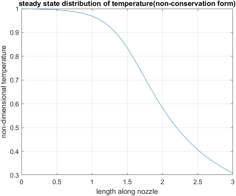
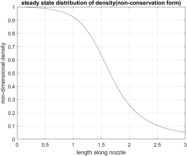
Steady state distribution of flow field variables with in the nozzle:
Non-conservation form:
Conservation form:
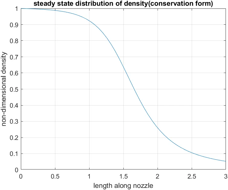
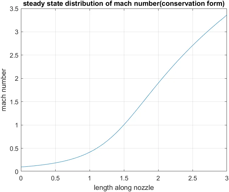
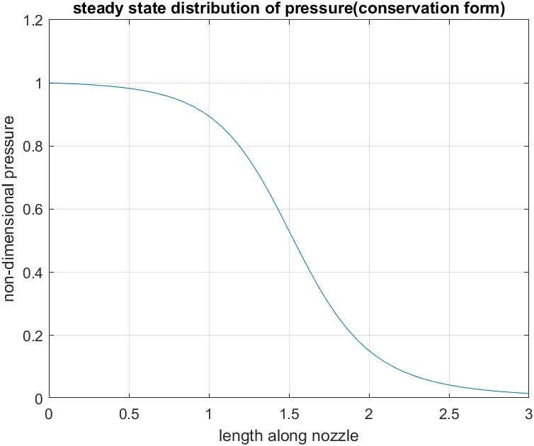
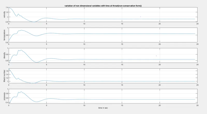
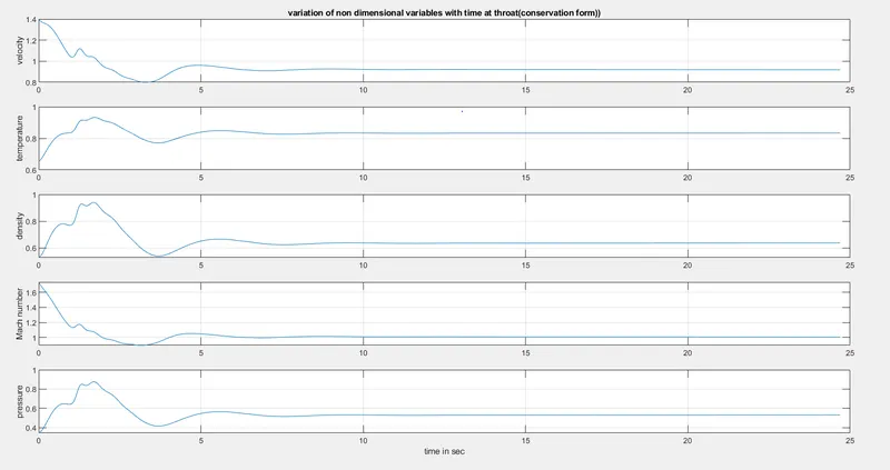
Time step variation of primitive variables at throat:
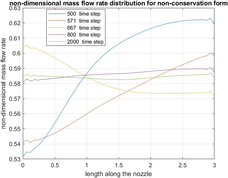
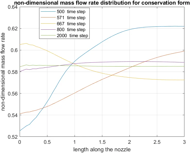
Variation of Mass flow rate distribution inside the nozzle at different time steps during the time-marching process:
Comparison of non-dimensionalised mass flow rate for non-conservation and conservation form:
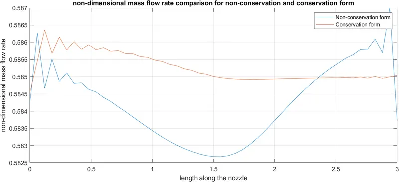
From the above plot, we note that the non-dimensionalised mass flow rate is almost constant for conservation form. This means, the conservation form is satisfying the conservation principles well. Hence the name.
Note: All the above plots are plotted with 51 grid points and 2000 time steps. The time steps are not equal, but calculated based on the stability criterion.
Grid dependency test:
For this purpose, let us compare steady state results at throat for both non-conservation and conservation forms at n=51 and n=101.
The results are tabulated for comparison in the below table:
| temperature | velocity | mach number | density | pressure | mass flow rate | |||||||
| n=51 | n=101 | n=51 | n=101 | n=51 | n=101 | n=51 | n=101 | n=51 | n=101 | n=51 | n=101 | |
| non-conservation form | 0.8355 | 0.8348 | 0.9138 | 0.9139 | 0.9998 | 1.0003 | 0.6376 | 0.6366 | 0.5327 | 0.5315 | 0.5827 | 0.5818 |
| conservation form | 0.835 | 0.8344 | 0.9139 | 0.9146 | 1.0047 | 1.0012 | 0.6402 | 0.6368 | 0.5345 | 0.5314 | 0.585 | 0.5824 |
From the above table, we can see that there is variation of flow field variables with the change in the number of nodes. Therefore, we can conclude that, the solution is grid dependent. However, this depends on the accuracy we are expecting.