Week 9 - Parametric study on Gate valve.

Aim:

To do a parametric study on the flow in a gate valve so that the velocity contour, velocity vector, and flow coefficient can be seen and calculated for each case. We will do a parametric study starting with the valve open at 10 mm and gradually increasing the opening by 10 mm until the valve is open at 80 mm.

Introduction:

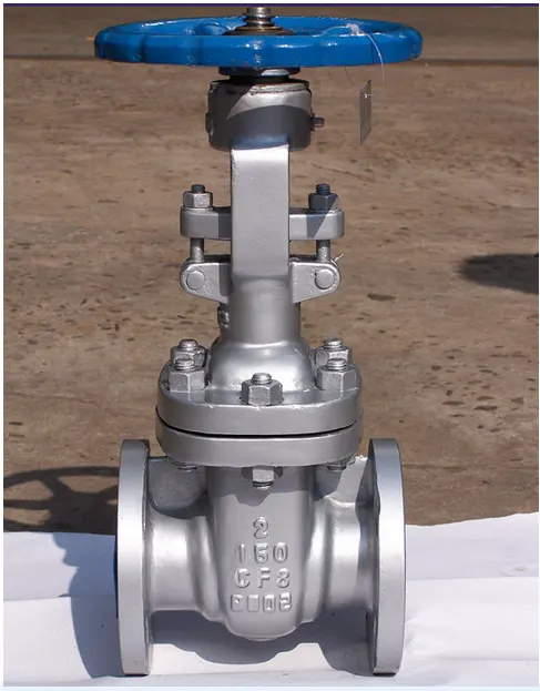
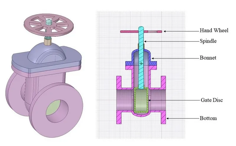
• A gate valve, which is also called a sluice valve, is a valve that lets fluid through when a barrier (the gate) is moved out of the way. Gate valves take up very little space along the axis of the pipe, and when the gate is fully open, they don't really stop the flow of fluid. The gate faces can be parallel, but most of the time they are in the shape of a wedge (in order to be able to apply pressure on the sealing surface).
• Instead of controlling the flow of liquids, gate valves are used to stop the flow of liquids. When the gate valve is fully open, there is nothing in the flow path, so the resistance to flow is very low. As the gate is moved, the size of the open flow path changes in a way that is not linear. This means that the flow rate doesn't change in a smooth way as the stem moves. Depending on how it is built, fluid flow can cause a partially open gate to shake.
• Most gate valves have a threaded stem that connects the actuator (such as a handwheel or motor) to the gate. Depending on which end of the stem is threaded, they have either a stem that rises or one that doesn't. Rising stems are attached to the gate. As the valve is turned, they rise and fall together, showing the position of the valve. The actuator is connected to a nut on the threaded stem. To move the actuator, the nut is turned around the stem. Non-rising stem valves are attached to the actuator and turn with it. They have a threaded gate that fits into the actuator. Since the gate moves inside the valve, they may have a pointer screwed onto the stem to show where the valve is. When there isn't much room up high, non-rising stems are used.
• Gate valves can have flanged ends that are drilled to meet standards for flange dimensions that work with pipelines.
• Most gate valves are made of cast iron, cast carbon steel, ductile iron, gunmetal, stainless steel, alloy steels, or forged steels.
• In ultra-high vacuum chambers, all-metal gate valves are used to seal off parts of the chamber.
• 

Solving and Modeling approach:

• Following the objectives, we will solve for 8 different scenarios. We are going to use the ANSYS Fluent solver to create the fluid volume in geometry and perform tetra CFD mesh with boundary definitions. After that, we will set up the physics of fluid flow and run the iterations to get solutions. Finally, we will use post processing to interpret the data in the form of plots, contours, vectors, streamlines, and other such things.
• We are going to analyze the mass flow rate at the outlet for eight different scenarios in which the valve disc lift position ranges from 10 mm to 80 mm with increments of 10 mm between each scenario.
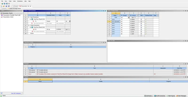
• In order to facilitate the execution of each and every scenario within the ANSYS Workbench's project schematic window, we will be utilizing the parametric set option for this kind of issue.
• We will need to keep in mind that we are working with a student edition of ASNYS, which means that the number of items with which we can experiment is restricted. The next step in the validation process involves tabulating the outcomes of the case study and comparing them with the findings of the published literature or book data.

Setting up the Preprocessor and the Solver:

• Let us open ANSYS workbench, now opening You can either double click on the Fluent button or use the drag-and-drop feature in the schematic window to create fluid flow. The fluent workflow is broken down into a series of steps, such as GEOMETRY > MESH > SETUP > SOLUTION > RESULTS. It is necessary to finish each stage before moving on to the next one so that the process can begin.

Case 1 is going to be considered, and we are going to talk about it in detail,

GEOMETRY >

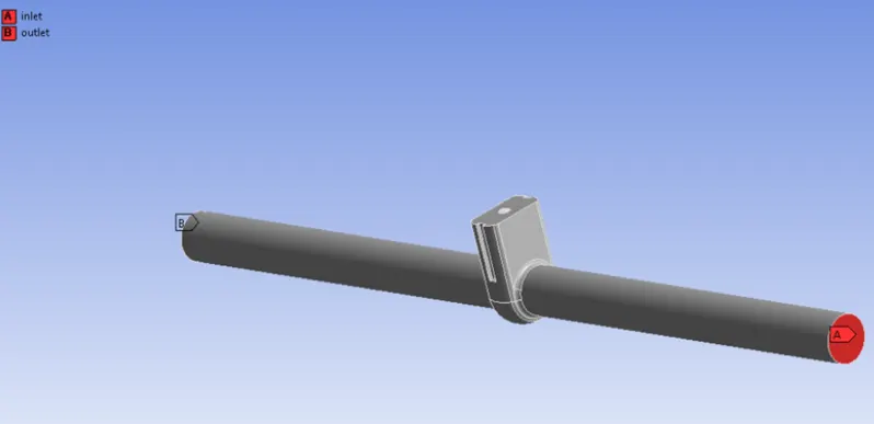
• To create a new SpaceClaim Geometry in the Fluent, right-click on the Geometry icon, and then select the option. When the space claim application loads, go to the File menu and select Open. Then, launch the Gate valve simulator. We are going to expand both faces to a total of 800 mm on each side by using the Pull tool.
• To obtain the fluid volume, go to the Prepare tab and pick the Volume extract option. Then, to obtain the fluid volume, select the margins of the inlet and outflow, as well as the edge that is close to the bonnet.
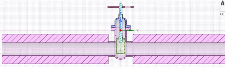
• After the fluid volume has been created, we can use the Move tool to select the disc, then move it in a positive z direction while inputting 10 millimetres of distance. Now within Groups, we have the opportunity to create a parameter, which we can use to turn it into an input parameter. Following this step, we will use the right mouse button to choose the volume, then we will click the Update volume by context option to bring the volume up to date with the new disc position.
• Because the solid volume is not required for the solving process, we can use the option to "suppress for physics" in order to view only the fluid volume in the physics section.
• We are good to go now. As soon as the geometry is available, we are able to close the space claim and verify that the fluid flow geometry has been changed, as indicated by a green tick.

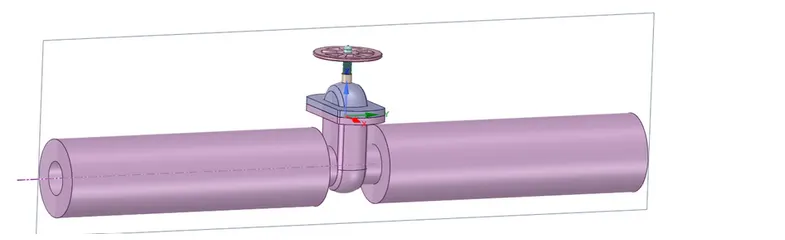
Gate disc partially opened

MESH >

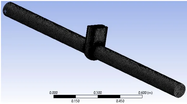
• The Mesh window can be opened by selecting edit from the context menu after right-clicking on the Mesh. Because the Mesh window is already loaded with the geometry that we have been working on, pressing the GENERATE MESH button ought to cause an automated generation of a mesh.
• The default mesh size that this site uses is around 92 millimetres. The default mesh type for these elements is tetra CFD. After choosing the Inlet and clicking the N button, we will give the outlet the name outlet and name the Inlet the name inlet. In the event that any modifications are made, the user must click the update icon in order to bring the mesh information up to date; otherwise, an alert in the form of a lightning bolt will appear, requesting that the user update.
• When this is finished, we should notice a green tick somewhere close to Mesh. It is possible for us to shut the mesh window.
• 
• 

Set up:

1. Solver: Steady

2. Type: Pressure Based

3. Gravitational Acceleration:

• X: 0
• Y: 0
• Z: -9.81 m/s²

4. Turbulence Model: k- epsilon with RNG

5.Cell Zone Condition:

• Fluid: Water

6. Material Specifications:

• Material: water-liquid (H₂o)
• Density: 998.2 Kg/m³
• Viscosity: 0.001003 Kg/m-s

6. Boundaries:

• Inlet: Pressure = `20 Pa(Gauge Pressure)`
• Outlet: Pressure= 0 Pa (Gauge Presssure)

7. Solution Methods: Coupled

8. Initialization:

• Method: Standard Initialization from the Inlet
• Number of Iteration: 300

SOLUTION >

• As a result of the fact that portion of the solution is calculated in the setup itself, we can see the green ticks in both the setup and the solution as well.

RESULTS >

• If you click the Results with the right mouse button, the Post processor should open. The default view is a wireframe model, and we can generate a plane on the YZ axis in order to observe contour. In a manner analogous to that of setup and solution, all plots and contours can be generated in this section.
• For Cases 2 through 8, we may adjust the disc lift position in the parameter set itself to be anywhere from 20 to 80 millimetres, and the results will be updated when we right-click and select "update chosen design points." In a later stage of post-processing, we will be able to construct contours, streamlines, and so on.

RESULTS:

• Following the execution of the same simulation methods across all of the cases derived from aim, we now have a number of data that can be compared and investigated. We are going to organize all of the contours, plots, and vectors so that we can examine them side by side and reach a decision. Only the outcomes of all of the examples are shown here; the inferences and interpretations based on those results will be briefly reviewed before the conclusion.

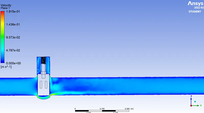
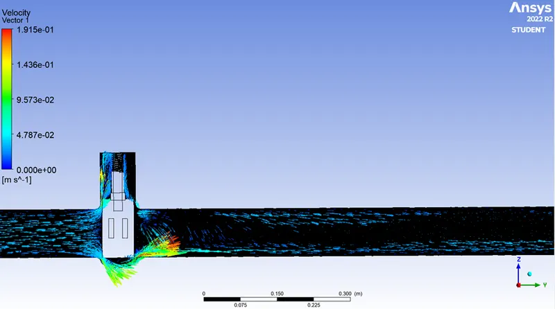
Case 1: Disc position at 10 mm

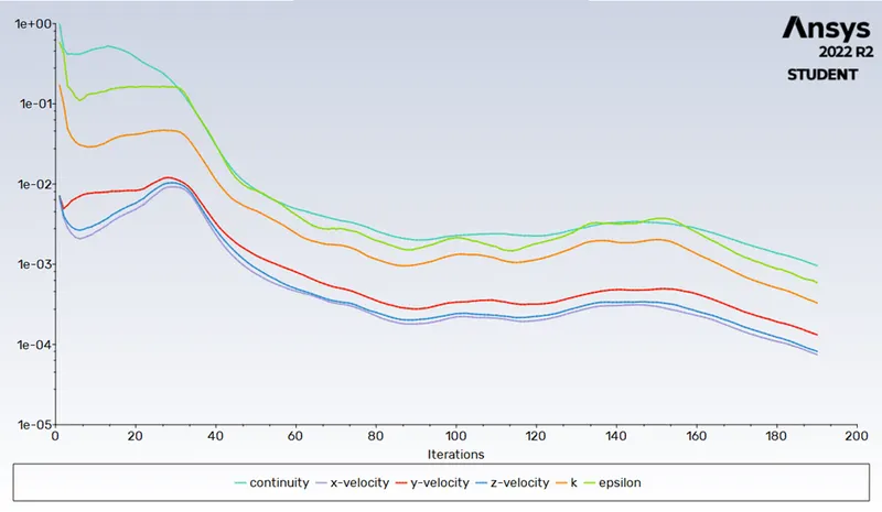
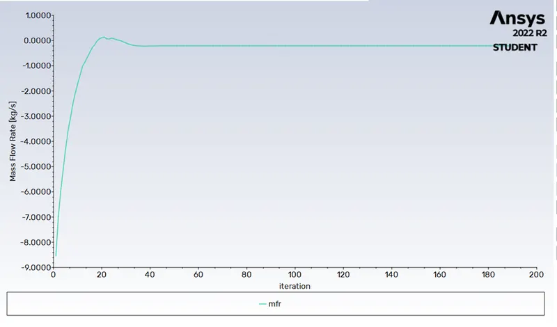
Residual & MFR Plot

Velocity contour

Velocity vector

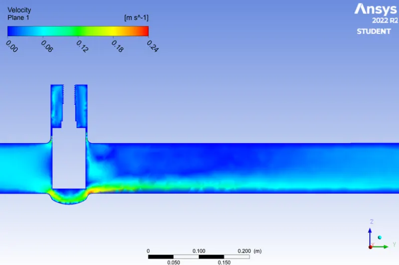
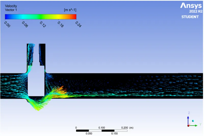
Case 2: Disc position at 20 mm

Velocity contour

Velocity vector

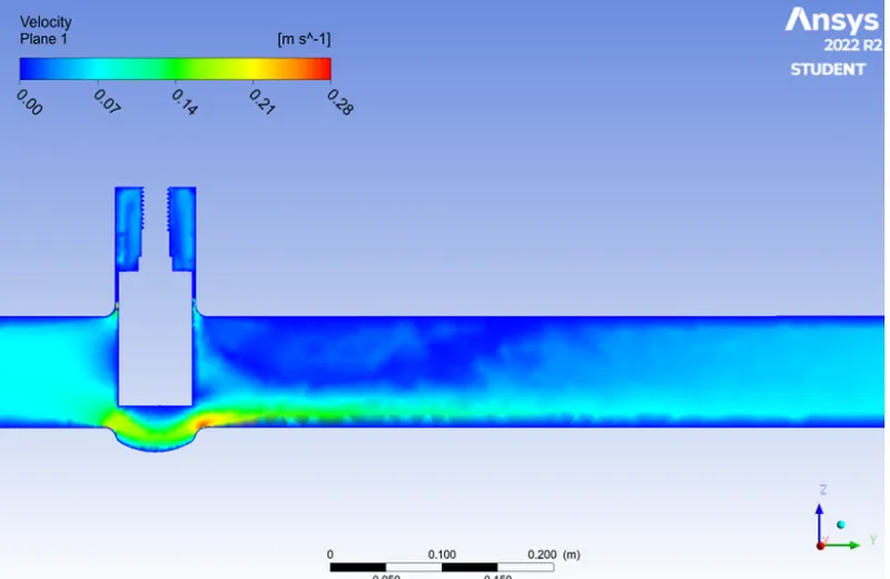
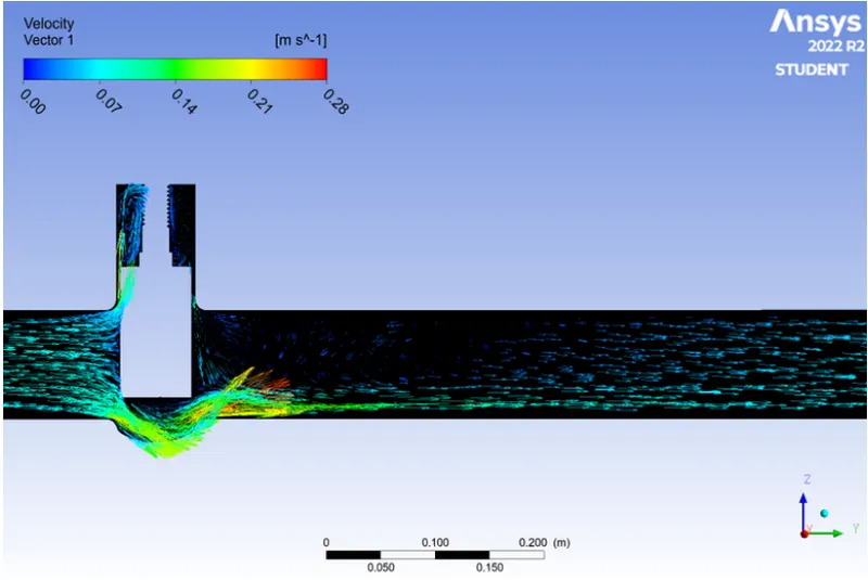
Case 3: Disc position at 30 mm

Velocity contour

Velocity vector

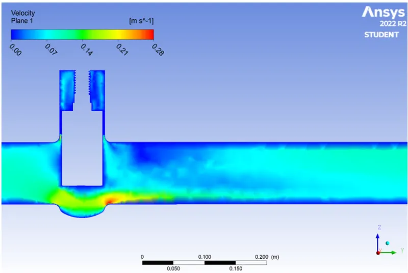
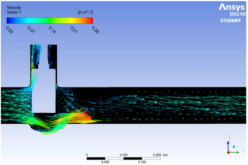
Case 4: Disc position at 40 mm

Velocity contour

Velocity vector

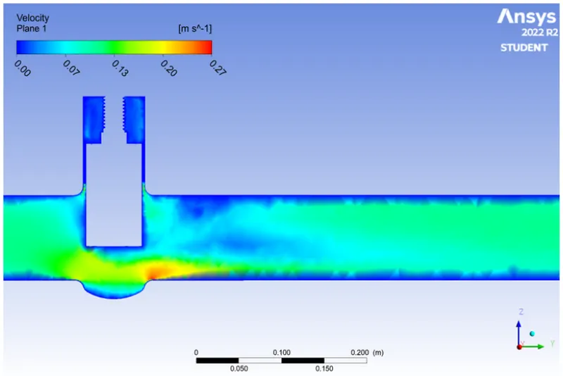
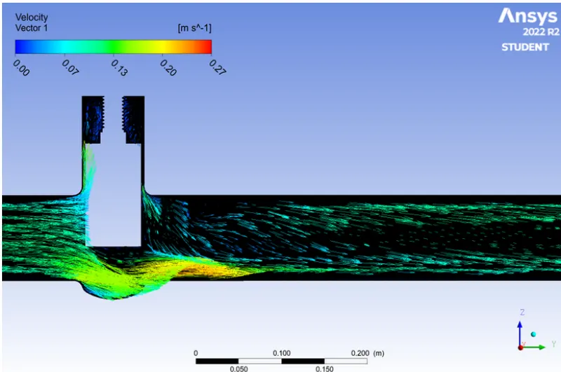
Case 5: Disc position at 50 mm

Velocity contour

Velocity vector

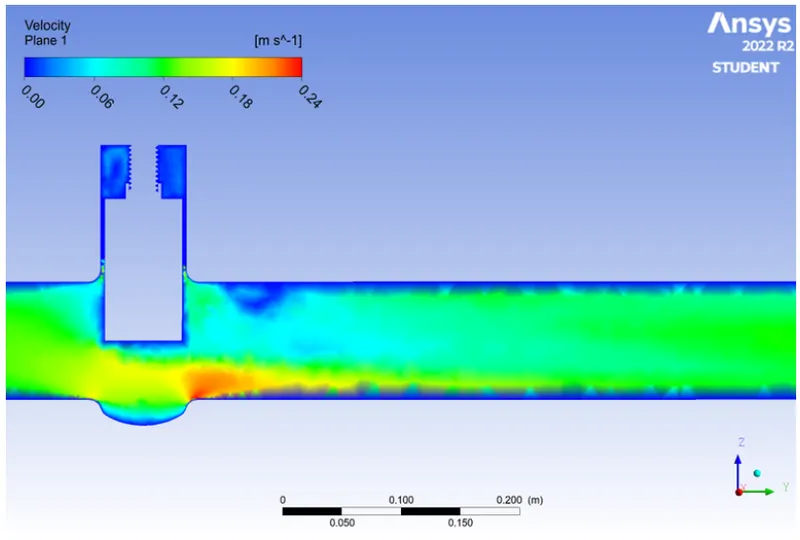
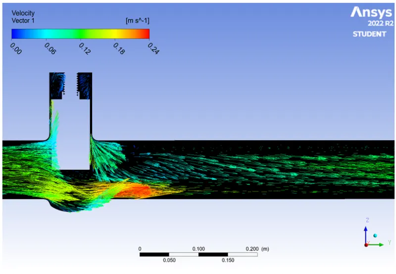
Case 6: Disc position at 60 mm

Velocity contour

Velocity vector

Case 7: Disc position at 70 mm

Velocity contour

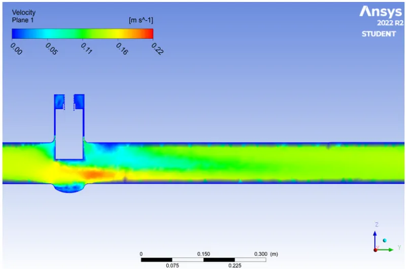
Velocity vector

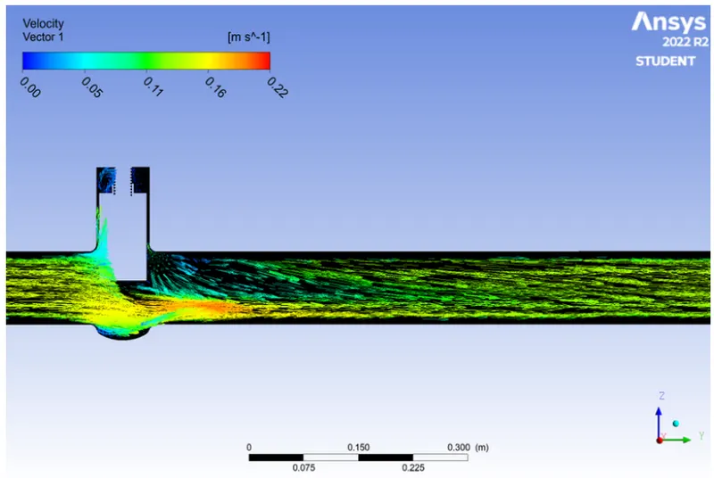
Case 8: Disc position at 80 mm

Velocity contour

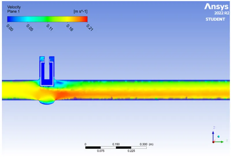
Velocity vector

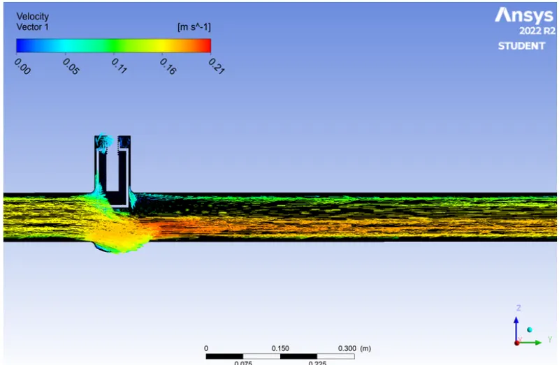
Mass Flow rate at each Design points (cases)

Flow-Factor(kv):

In metric terms, the flow coefficient is denoted by the letters Kv. It is measured in cubic metres per hour (m3/h) and takes place when the temperature of the water is 16 degrees Celsius and there is a pressure drop of one bar across the valve. The flow coefficient is denoted by the symbol Cv when using imperial units.

Flow-coefficient(Cv):

The coefficient of flow, often known as Cv, is a formula that may be used to determine the flows that a valve produces under different situations. This formula can also be used to choose the appropriate valve for a flow application. The Cv was developed for use with liquid flows; it describes the flow in gallons per minute of water at a temperature of sixty degrees Fahrenheit with a pressure drop across the valve of one pound per square inch.

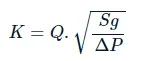
K = Cv , when k is referenced in [gpm] [psi] unit

K = Kv , when k is referenced in [m3/hr] [bar] unit

where Q = mass flow rate

Sg = Specific gravity of water which is equal to 1

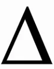P = Change in pressure or pressure drop across valve

Relation between Kv and Cv:

Cv = Kv*1.156

CONCLUSION:

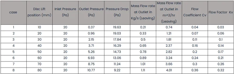
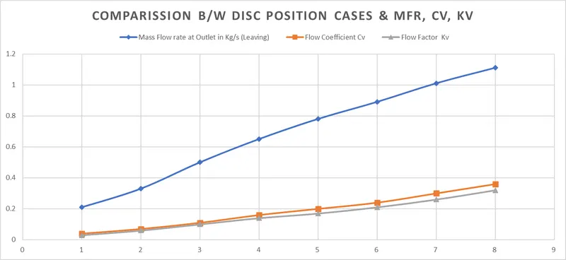
• The results of the parametric analysis presented above, along with all of the plots, make it abundantly clear that an increase in the mass flow rate at the outflow may be expected if the disc position is increased from 10 mm to 80 mm. In addition, the values of the flow factor and the flow coefficient are consistent with one another.
• The interesting part about the venturi effect at the disc is that it gives birth to increased velocity in cases 0.18 to 0.28 m/s and lowers to 0.22 m/s in 80 mm open state. This happens for every step increase in the number of instances.
• Because the maximum velocity occurs at the disc exit radius zone (as determined by the velocity contour), that region is susceptible to surface abrasion over the long term. Therefore, the material that was utilised has a significant influence in deciding how long the valve will last. Let's say that under high pressure inlet conditions, we can employ gun metal valves rather than cast iron valves.

INFERENCES:

• When the disc opens up more, there is a greater rate of mass flow at the outflow.
• For the system to run smoothly, it is critical to regularly update the volume that is being claimed in spaceclaim by context.
• When case by case is applied, the total pressure at the outlet rises in a manner that is proportionate to the disc lift position.
• Utilizing a parametric study saves a lot of time because it eliminates the need to open the fluent spreadsheet for each individual scenario.
• Because of the venturi effect, the velocity at the disc exit can both rise and decrease depending on the circumstances.