Week 3 - Solving second order ODEs

Aim:

To solve second order ODE using MATLAB Programming

Objective:

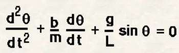
1. To write a program that solves the following ODE. This ODE represents the equation of motion of a simple pendulum with damping.
2. To create Animation of Pendulum.

EQUATIONS USED:

Where as,

g = gravity in m/s2,

L = length of the pendulum in m,

m = mass of the ball in kg,

b=damping coefficient.

The body of content

ODE MAIN CODE:

clear all
close all
clc

b = 0.05
g = 9.81
l = 1
m = 1

%Intial condition
theta_0 =[0;3];

% time points
t_span = linspace(0,20,500);

% solve ODE
[t, results] = ode45(@(t,theta) ode_func(t, theta, b,g,l,m),t_span,theta_0);

figure(1)
plot(t,results(:,1))
hold on
plot(t,results(:,2))
xlabel('time')
ylabel('plot')
grid on;

%Animation
theta1 = results(:,1);
ct = 1; % counter actually represents each and every frame

 for i=1:length(theta1)
     r = theta1(i);
     x0=1;
     y0=1; 
     x1=1 -l*sin(r);
     y1=1 -l*cos(r);

     figure(2)
     plot([0 2],[1 1], 'linewidth',4,'color','g');
     axis([-2 5 -2 2]);
     hold on
     plot([x0 x1],[y0 y1],[x1 x1],[y1 y1],'o','MarkerSize',20,'color', 'r')
     title('Damping of Pendulum');
     legend('Support rod','length of pendulum','Bob of pendulum');
     grid on;
     hold off;
     pause(0.02)
     M(ct) = getframe(gcf);
     ct=ct+1;
 end

movie(M);
videofile = VideoWriter('pendulum.avi','Uncompressed AVI');
open(videofile);
writeVideo(videofile,M);
close(videofile);

ODE_FUNC Program:

function [dtheta_dt]= ode_func(t,theta,b,g,l,m)


theta1 = theta(1)
theta2 = theta(2)
dtheta1_dt = theta2;
dtheta2_dt = -(b/m)*theta2 - (g/l)*sin(theta1);
dtheta_dt = [dtheta1_dt; dtheta2_dt];

end

EXPLANATION:

1. By providing the initial inputs that includes the value of b, g, l & m.
2. Following with initial inputs, While solving the ODE system, two first order ODE, first describes the initial displacement and second describes the initial velocity in 3 m/s
3. Here inbuilt solver in MATLAB ode45 used to solve the second order ODE.
4. Since ode45 can only solve a first order ode, the pendulum equation has to be converted into two first order ODE as defined in the separate generated function program named “ode_func”.
5. Here, t & theta are the function. Where as "ode_func(t, theta, b, g, l, m" says how your ode function is defined by calling the sepearte ode function (attached).
6. After defining everything now plot command is used to generate figure as usual.
7. 
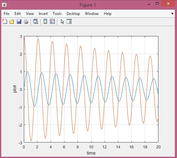
8. Here blue line represents the displacement & red line represent the velocity.

9. After doing this, now creating animation we need to use for loop command. But before that Ct comand will be used.

10. For loop command with using I to length theta1 and.

11. However, “theta” is an array.

12. Adding all mathematical expressions mentioning the values of x0,x1, y0,y1

13. After that using Plotting command where plots are being used instead of giving line command. As plots will give clear animation.

14. Mentioning axis with [-2 5 -2 2] will give the clear animation within the mentioned axis boundary which will look elegant also.

15. Here,counter actually represents each and every frame. we create an array called “M” while making movie/animation. At the last te video dmesify the position of pendulum.

    Link of youtube for pendulum.

    https://youtu.be/dcyB13HszGw

Conclusion:

We can say that by increasing the value of damp coef, the oscillation damp quickely.

Not only tis but all te factor also effect the final output if we are changing the value of b g l m.