Week 4.1 - Genetic Algorithm
Aim: To optimize the staglagmite function using genetic algorithm techniques using MATLAB
The following ideas must first be understood in order to develop the genetic algorithm:
1.) What is a genetic algorithm?
2.) How genetic algorithm work using syntax.
Genetic algorithm:
The genetic algorithm is a method based on natural selection, the process that drives biological evolution, for addressing both limited and unconstrained optimization problems. The population size of distinct solutions is always changing thanks to the evolutionary algorithm.
Charles Darwin's notion of natural evolution serves as the inspiration for a search experience known as a genetic algorithm. By selecting the best individuals for reproduction in order to create the next generation's children, this algorithm mimics the process of natural selection.
Phases in Genetical Algorithm
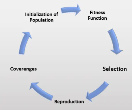
A.) Intialization of Population:
Each gene stands for a parameter (variable) in the response. The chromosome is this set of variables that makes up the solution. As a result, the population is made up of chromosomes.
It concerns which genes are on each chromosome.
Although chromosomes are frequently represented as binary 0s and 1s, there are several alternative encodings.
B.) Fitness Function
Out of the available chromosomes, we must choose the finest ones to create kids, hence each chromosome is assigned a fitness value.
The fitness rating is useful in choosing the people who will be employed for reproduction.
C.) Selection
Finding the area where getting the greatest answer is more likely is the major objective of this phase.
The survival of the fittest served as inspiration for this. Exploration and utilisation of the search space ought to be balanced. In the search space, GA aims to shift the genotype to a higher fitness level. Solutions that are less than ideal can result from a significant fitness selection bias. A search that is not narrowed down enough through fitness bias selection is unfocused.
In order to choose potentially beneficial recombination solutions, fitness proportional selection—also known as roulette wheel selection—is employed as a genetic operator in genetic algorithms.
D.) Reproduction
Generation of offsprings happen in 2 ways:
- Crossover
- Mutation
a) Crossover
Crossover is the most vital stage in the genetic algorithm. During crossover, a random point is selected while mating a pair of parents to generate offsprings.
There are 3 major types of crossover.
Single Point Crossover: A point on both parents’ chromosomes is picked randomly, and designated a ‘crossover point’.
Two-Point Crossover: Two crossover points are picked randomly from the parent chromosomes.
Uniform Crossover: In a uniform crossover, typically, each bit is chosen from either parent with equal probability. The new offspring are added to the population.
b) Mutation
Some of the newly produced offspring's genes may be subject to a low-probability mutation. This suggests that some bits on the bit chromosome can be switched around. Mutation occurs to maintain population variety and prevent early convergence.
E.) Convergence (when to stop)
Following are a few guidelines that can help you determine when to stop:
- when a predetermined number of generations have been completed and there has been no progress in the quality of the answer.
- when a fixed number of generations and years are reached.
- until a workable resolution is found.
Syntax for GA:
[x,fval ,exitflag ,output ,population ,scores]= ga(func,nvars,A,b,Aeq,Beq,lb,ub,nonlcon,Intcon,options)
x = optimum solution
exitflag = reason ga stopped
output= information about optimization process
population=final population
scores= final scores
f=ga(fun,nvars,A,b,[],[],lb,ub,nonlcon,IntCon,options)
fun - fitness function.
nvars- number of variables,
A,b= Linear inequality constraints
Aeq,beq=Linear equality constraints
lb- Lower bound(limit),
ub- Upper bound(limit),
nonlcon : Use for nonlinear constraints
IntCon : to get solution in integer.
options- To set population size minimize with non-default options.
BODY OF THE CONTENT:
- FITNESS FNUCTION
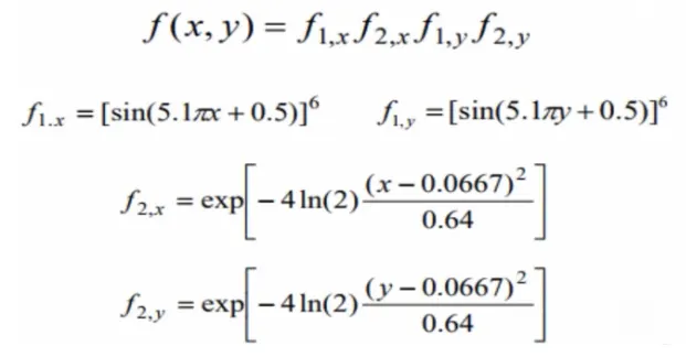
The stalagmite function in the primary functions uses the aforementioned formulae to plot the graph.
Function Code:
function [f] = stalagmite(input_vector)
x = input_vector(1);
y = input_vector(2);
f1x = (sin(5.1*pi*x + 0.5))^6;
f1y = (sin(5.1*pi*y + 0.5))^6;
f2x = exp((-2.7726)*(x-(0.0667))^2/0.46);
f2y = exp((-2.7726)*(y-(0.0667))^2/0.46);

f = -(f1x*f1y*f2x*f2y);
end
1.) Stalagmite function code:
clear all
close all
clc

%Defining our search space
x = linspace(0,0.6,150);
y = linspace(0,0.6,150);
num_case = 60;

%creating a 2Dimensional mesh
[xx yy] = meshgrid(x,y);

%Evaluating the stalagmite function

for i = 1:length(xx)
    for j = 1:length(yy)
        input_vector(1)=xx(i,j);
        input_vector(2)=yy(i,j);
        f(i,j) = stalagmite(input_vector);
    end
end

tic
for k = 1:num_case;
    [inp, fval(k)] = ga(@stalagmite,2);
    x_1(k) = inp(1);
    y_1(k) = inp(2);
end
study1_time = toc

figure (1)
hold on
grid on
surfc(xx,yy,-f)
shading interp
title('stalagmite plot')
xlabel('X')
ylabel('Y')

figure(2)
subplot(2,1,1)
surfc(xx,yy,-f)
shading interp
hold on
plot3(x_1,y_1,-fval,'marker','o','MarkerSize',5,'MarkerFaceColor','m')
title('unbounded inputs')
subplot(2,1,2)
plot(-fval)
xlabel('iterations')
ylabel('function minimum')
RESULTS for basic stalagmite function and case study (I)
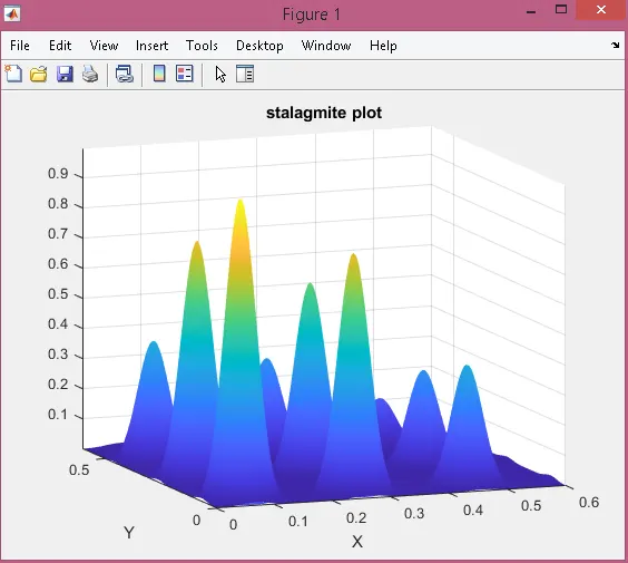
figure (1) - stalagmite basic
As we can see, there are more peaks that are developing upward, which essentially make up my stalagmite structure. However, the function typically returns a negative value, which corresponds to local minima; therefore, to obtain both local and global maxima, the function must be made positive. peaks that are upgrowing Global maxima, the tallest peak, and local maxima are other peaks.
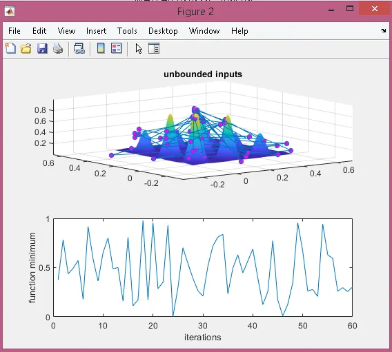
figure(2)- case study (I)
Since the solutions in this case study (I) are not bounded, the GA will determine all feasible maxima in 'x' and 'y' coordinates. and it takes 6.4665 seconds to calculate the potential solution.
study(II)
Since the answer is scattered across space, we restrict it to the global maxima by converging the area for the GA function to the best values. By repeating the for loop 50 times, we are improving our solution to produce better results from generation to generation.
MATLAB CODE(II)
% 2nd case study statistical behaviour
tic
for s = 1:num_case;
    [input,fval(s)]= ga(@stalagmite,2,[],[],[],[],[0,0],[0.6,0.6]);
    x_2(s)= input(1);
    y_2(s)= input(2);

end
study2_time = toc;
figure(3)
subplot(2,1,1)
surfc(xx,yy,-f)
shading interp
hold on
plot3(x_2,y_2,-fval,'marker','o','MarkerSize',5,'MarkerFaceColor','m')
title('unbounded inputs')
subplot(2,1,2)
plot(-fval)
xlabel('iterations')
ylabel('function minimum')
RESULT
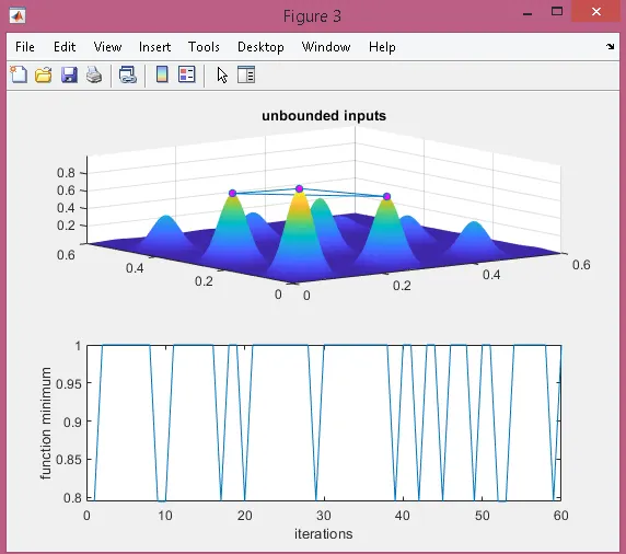
In case 2nd we can observe that, the time required in study two's result for reading global maxima is 8.6754. Here, we're utilising a genetic algorithm tool to limit the lower and upper values since, if we do, the ga tool will only search inside those bounds. Here, the lower and upper bounds for the x and y directions are assumed to be 0 and 0.6, respectively.
case study (III)
MATLAB CODE
% 3rd case study increasing ga iterations
options = optimoptions('ga');
options = optimoptions(options,'PopulationSize',500);

tic
for m = 1:num_case;
    [input,fval(m)]= ga(@stalagmite,2,[],[],[],[],[0,0],[0.6,0.6],[],[],options);
    x_3(m)= input(1);
    y_3(m)= input(2);

end
study3_time = toc
figure(4)
subplot(2,1,1)
surfc(xx,yy,-f)
shading interp
hold on
plot3(x_3,y_3,-fval,'marker','o','MarkerSize',5,'MarkerFaceColor','m')
title('unbounded inputs')
subplot(2,1,2)
plot(-fval)
xlabel('iterations')
ylabel('function minimum')
RESULT
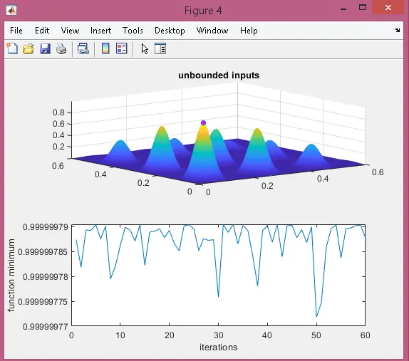
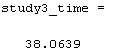
The value of the variation range has significantly changed in the situation mentioned above, as can be seen.
NOW THE FINAL PROGRAM AT ONCE FOR THREE STUDIES:-
clear all
close all
clc

%Defining our search space
x = linspace(0,0.6,150);
y = linspace(0,0.6,150);
num_case = 60;

%creating a 2Dimensional mesh
[xx yy] = meshgrid(x,y);

%Evaluating the stalagmite function

for i = 1:length(xx)
    for j = 1:length(yy)
        input_vector(1)=xx(i,j);
        input_vector(2)=yy(i,j);
        f(i,j) = stalagmite(input_vector);
    end
end

tic
for k = 1:num_case;
    [inp, fval(k)] = ga(@stalagmite,2);
    x_1(k) = inp(1);
    y_1(k) = inp(2);
end
study1_time = toc

figure (1)
hold on
grid on
surfc(xx,yy,-f)
shading interp
title('stalagmite plot')
xlabel('X')
ylabel('Y')

figure(2)
subplot(2,1,1)
surfc(xx,yy,-f)
shading interp
hold on
plot3(x_1,y_1,-fval,'marker','o','MarkerSize',5,'MarkerFaceColor','m')
title('unbounded inputs')
subplot(2,1,2)
plot(-fval)
xlabel('iterations')
ylabel('function minimum')


% 2nd case study statistical behaviour
tic
for s = 1:num_case;
    [input,fval(s)]= ga(@stalagmite,2,[],[],[],[],[0,0],[0.6,0.6]);
    x_2(s)= input(1);
    y_2(s)= input(2);

end
study2_time = toc;
figure(3)
subplot(2,1,1)
surfc(xx,yy,-f)
shading interp
hold on
plot3(x_2,y_2,-fval,'marker','o','MarkerSize',5,'MarkerFaceColor','m')
title('unbounded inputs')
subplot(2,1,2)
plot(-fval)
xlabel('iterations')
ylabel('function minimum')

% 3rd case study increasing ga iterations
options = optimoptions('ga');
options = optimoptions(options,'PopulationSize',500);

tic
for m = 1:num_case;
    [input,fval(m)]= ga(@stalagmite,2,[],[],[],[],[0,0],[0.6,0.6],[],[],options);
    x_3(m)= input(1);
    y_3(m)= input(2);

end
study3_time = toc
figure(4)
subplot(2,1,1)
surfc(xx,yy,-f)
shading interp
hold on
plot3(x_3,y_3,-fval,'marker','o','MarkerSize',5,'MarkerFaceColor','m')
title('unbounded inputs')
subplot(2,1,2)
plot(-fval)
xlabel('iterations')
ylabel('function minimum')
Conclusion: We obtained the stalagmite plot using simple MatLab methods. The stalagmite plot exhibits statistical behaviour. Using the GA tool, we then finalised our plot's optimization and advanced it to its crucial point in order to reach the global maxima. Additionally, we learned that expanding the population and iterating it led to the optimization of the stalagmite function produced by GA.
References: