Week 9 - Parametric study on Gate valve.

Week 9 - Gate valve Parametric study.

Aim:

To perform parametric study on flow in gate valve to visualize the velocity contour, velocity vector and calculate the flow co-efficient for each case. We shall perform parametric study from 10 mm valve open position to gradually increase the opening in units of 10 mm upto 80 mm valve open position.

Introduction:

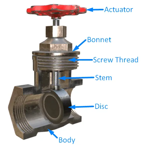
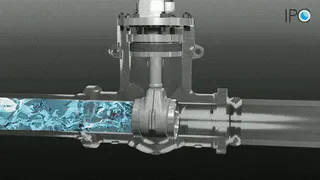
A gate valve, also known as a sluice valve, is a valve that opens by lifting a barrier (gate) out of the path of the fluid. Gate valves require very little space along the pipe axis and hardly restrict the flow of fluid when the gate is fully opened. The gate faces can be parallel but are most commonly wedge-shaped (in order to be able to apply pressure on the sealing surface).

Gate valves are used to shut off the flow of liquids rather than for flow regulation. When fully open, the typical gate valve has no obstruction in the flow path, resulting in very low flow resistance. The size of the open flow path generally varies in a nonlinear manner as the gate is moved. This means that the flow rate does not change evenly with stem travel. Depending on the construction, a partially open gate can vibrate from the fluid flow.

Construction : Common gate valves are actuated by a threaded stem that connects the actuator (e.g. hand wheel or motor) to the gate. They are characterized as having either a rising or a non rising stem, depending on which end of the stem is threaded. Rising stems are fixed to the gate and rise and lower together as the valve is operated, providing a visual indication of valve position. The actuator is attached to a nut that is rotated around the threaded stem to move it. Non rising stem valves are fixed to, and rotate with, the actuator, and are threaded into the gate. They may have a pointer threaded onto the stem to indicate valve position, since the gate's motion is concealed inside the valve. Non rising stems are used where vertical space is limited.

Gate valves may have flanged ends drilled according to pipeline-compatible flange dimensional standards.

Gate valves are typically constructed from cast iron, cast carbon steel, ductile iron, gunmetal, stainless steel, alloy steels, and forged steels.

All-metal gate valves are used in ultra-high vacuum chambers to isolate regions of the chamber.

Solving and Modeling approach:

We shall solve for 8 cases as discussed in Aim. We will be using ANSYS Fluent solver to create the fluid volume in geometry and perform tetra CFD mesh with boundary definitions, setup the physics of fluid flow and run the iterations to get solutions, using post processing to interpret the data in form of plots,contours, vectors, streamlines etc.,

we shall study for 8 cases with the valve disc lift position from 10 mm to 80 mm in increments of 10 mm each, and study the mass flow rate at the outlet.

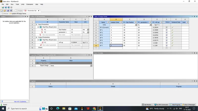
For this type of problem, we will be using parametric set option so that all cases can be run at the project schematic window of the ANSYS Workbench.

We shall keep in mind we are using a student version of ASNYS, so we are limited with the number of elements to play with. Then, we tabulate the case study results and compare it with the open literature or book data results to validate the simulation.

Preprocessing and Solver setting:

Let us open ANSYS workbench, now opening Fluent flow can be done by drag and drop in the schematic window or by double clicking on Fluent. The fluent workflow is in a series of steps such as GEOMETRY > MESH > SETUP > SOLUTION > RESULTS. Each step has to be completed for the next step to initialize.

we shall consider case 1 and discuss in detail,

GEOMETRY >

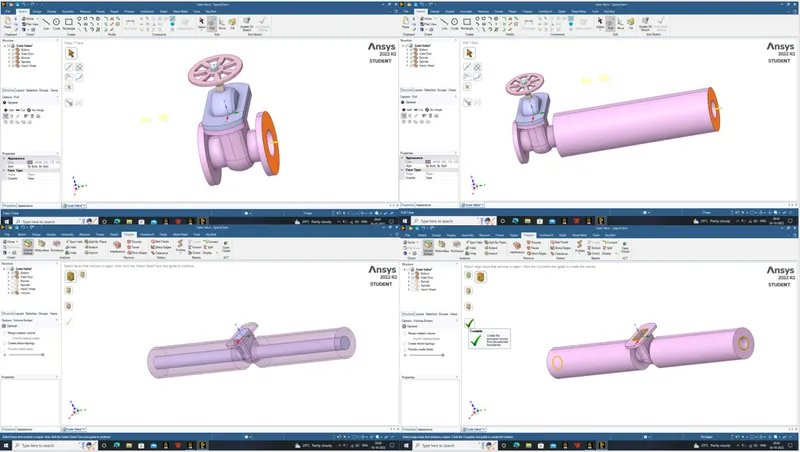
In the Fluent, right click on the Geometry and select New SpaceClaim Geometry. The space claim application opens, select FILE > OPEN and open the Gate valve model. Using the Pull tool, we shall extend both faces upto 800 mm each side.

In the Prepare tab, select the Volume extract option to extract the fluid volume and select the edges if inlet , outlet and the edge near the bonnet to extract the fluid volume.

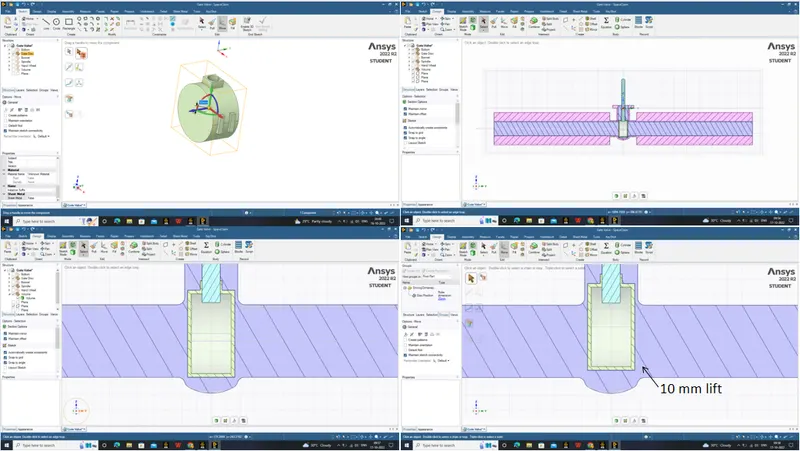
After fluid volume creation, we can use the Move tool to select the disc and move it in positive z direction and input 10 mm. Now in Groups we can select Create Parameter option to make it an input parameter. After this step, we shall select the volume and right click to select Update volume by context option to update the volume as per the new disc position.

We don’t need the solid volume for solving, so we can select the suppress for physics option to see only fluid volume in physics.

We are good to go now. Once the geometry is ready, we can close space claim and check that the fluid flow (fluent) geometry is updated indicated by a green tick.

MESH >

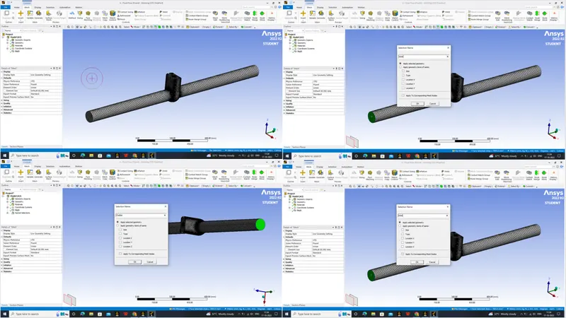
Right clicking on the Mesh and selecting edit opens the Mesh window. Mesh window is preloaded with the geometry we have worked on earlier, so clicking on the GENERATE MESH should create a mesh automatically.

The default mesh size here is 92 mm approx. The elements are tetra CFD mesh by default. Selecting the Inlet and clicking on N and we shall name as inlet and outlet as outlet respectively. Any changes made, click on the update icon to update the mesh details or else there is an indication of a thunderbolt sign asking the user to update.

Once this is done, we should see a green tick near Mesh. we can close the mesh window.

SETUP >

Right clicking on the Setup, opens the Fluent launcher. In the Fluent launcher select 3D, Double precision and select the number of cores as per the user system configuration and click on start.

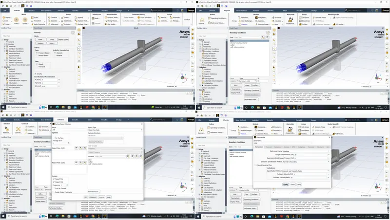
Upon opening, there are some selections to be done to define the simulation definitions, we shall select Type: Pressure based, Velocity Formulation: Absolute, Time: Steady, Gravity on in Z axis input -9.81 m/s^2. Under the Physics tab, we can turn on viscous and select k-epsilon > RNG > Swirl dominating flow as well.

Under the materials we shall select Water<liquid> as our default material.

In cell zone, change the default material as water and delete air in materials tab to avoid confusion.

In the Boundary conditions, select the inlet as pressure inlet and input pressure as 20 Pa (usual flow pressure) and select the nearby arrow button and select New parameter to create it as a new input parameter if required.

We need mass flow rate plot for outlet, the same can be created from Solution > Reports > New > Surface Report > Mass flow rate and select the outlet. Here, we shall check print to console as well as create output parameter so that Mass flow rate is displayed in the parameter set.

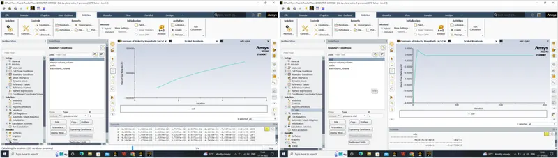
Now, it's time to start the simulation. For Run Calculation, we shall run for 350 iterations initially if required we shall extend based on the number of incomplete particles.

In the Outline view under Simulation Reports, clicking on the Report Outline > Generate should generate a Ansys Fluent Simulation Report which is automatically generated with all the information of the simulation in it. This can be exported as a PDF also. We are done with setup, we can close the setup.

SOLUTION >

Since some solution is calculated in the setup itself, we can see the green ticks in both setup and solution too.

RESULTS >

Right clicking on the Results should open the Post processor. Default view is a wireframe model, we can create a plane in YZ to view contour. Similar to setup and solution, all contours and plots can be created here, in addition to that we can create an animation of the velocity contour by clicking on AUTOSAVE during the solution and clicking on ANIMATE select make movie and save in desired location.

For Case 2 to 8 we can change the disc lift position in the parameter set itself as 20, 30, up to 80 mm and right click update selected design points will update the results. Later in post processing we can create contours, streamlines etc,..

RESULTS:

After repeating the similar manner of simulation procedures for all cases from aim, we have a handful of data to compare and study. We shall put in order all the contours, plots and vectors for us to compare and come to a conclusion. Here, only the results of all cases are displayed, its inference and interpretation shall be discussed briefly in conclusion.

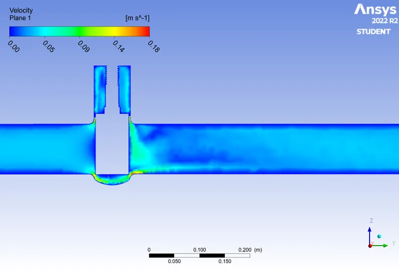
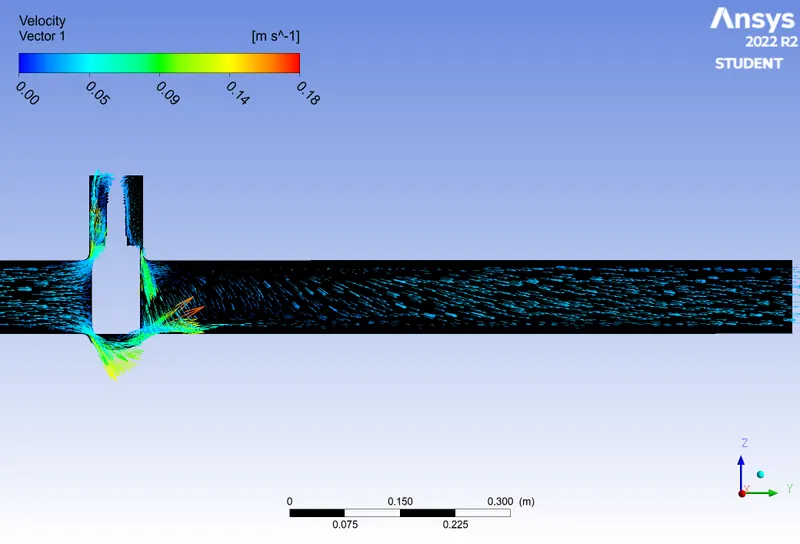
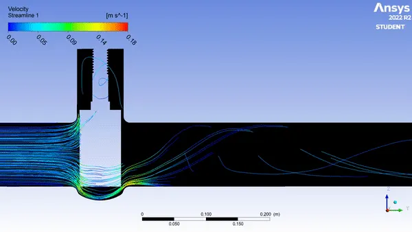
Case 1: Disc position at 10 mm

Velocity contour

Velocity vector

Animation of Streamline

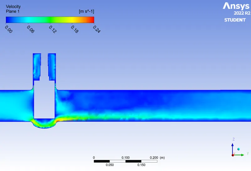
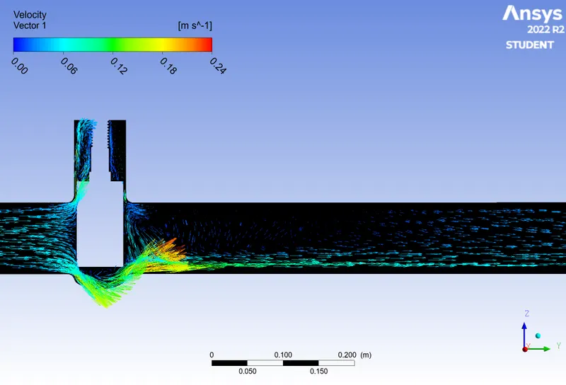
Case 2: Disc position at 20 mm

Velocity contour

Velocity vector

Animation of streamline

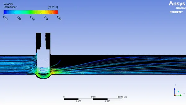
Case 3: Disc position at 30 mm

Velocity contour

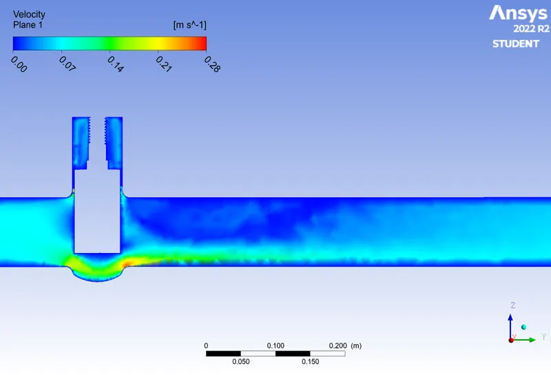
Velocity vector

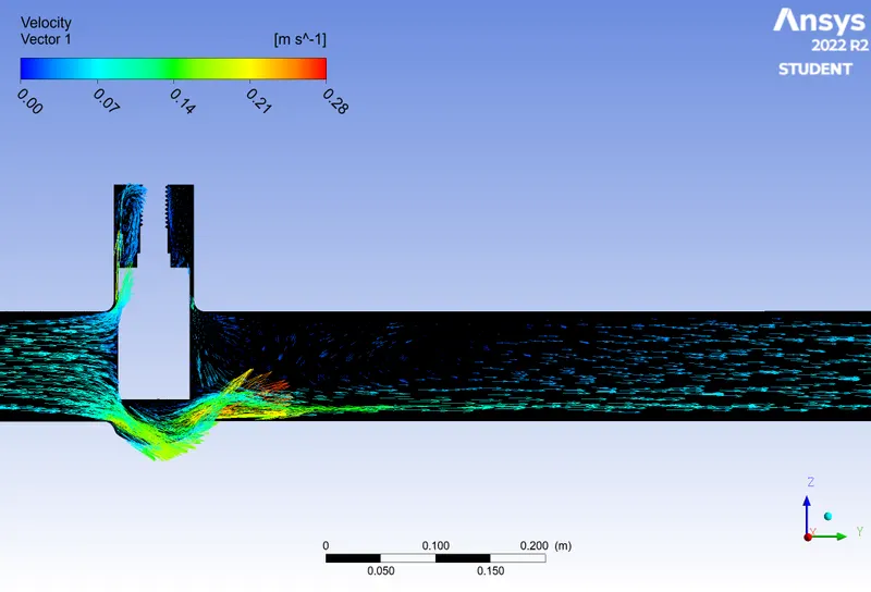
Animation of streamline

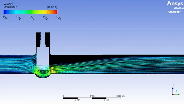
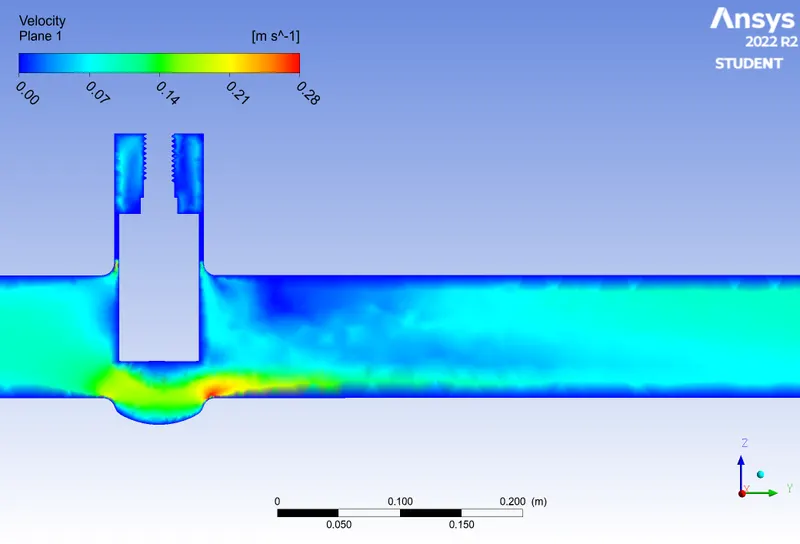
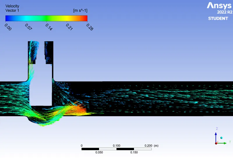
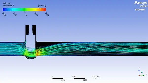
Case 4: Disc position at 40 mm

Velocity contour

Velocity vector

Animation of streamline

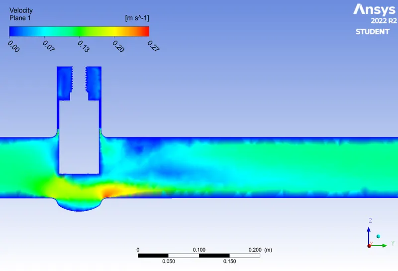
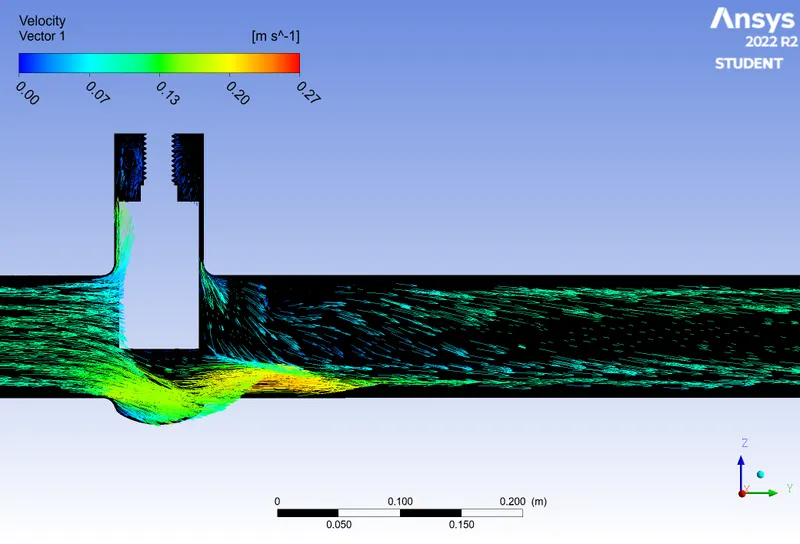
Case 5: Disc position at 50 mm

Velocity contour

Velocity vector

Animation of streamline

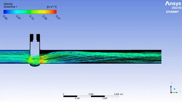
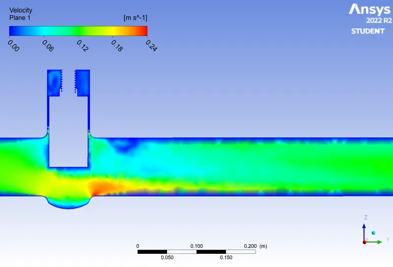
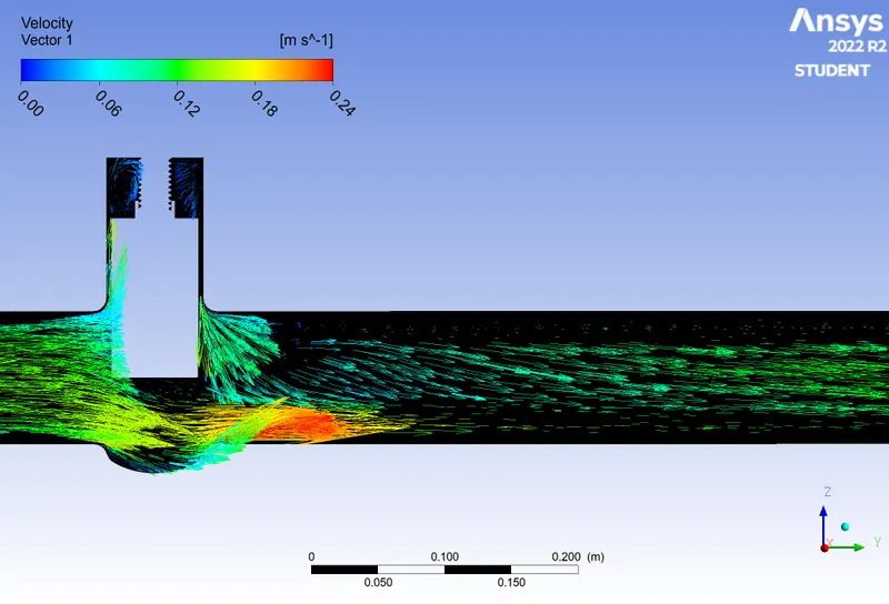
Case 6: Disc position at 60 mm

Velocity contour

Velocity vector

Animation of streamline

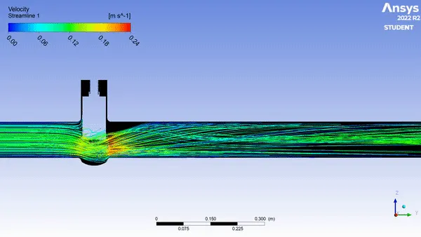
Case 7: Disc position at 70 mm

Velocity contour

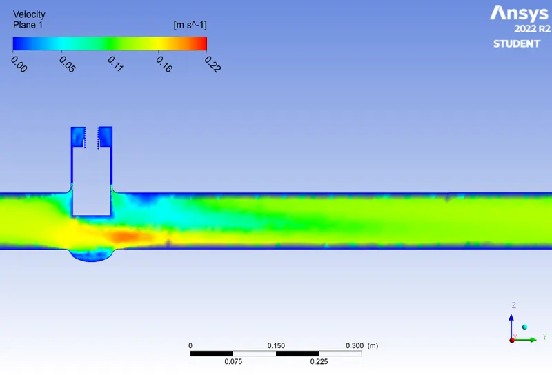
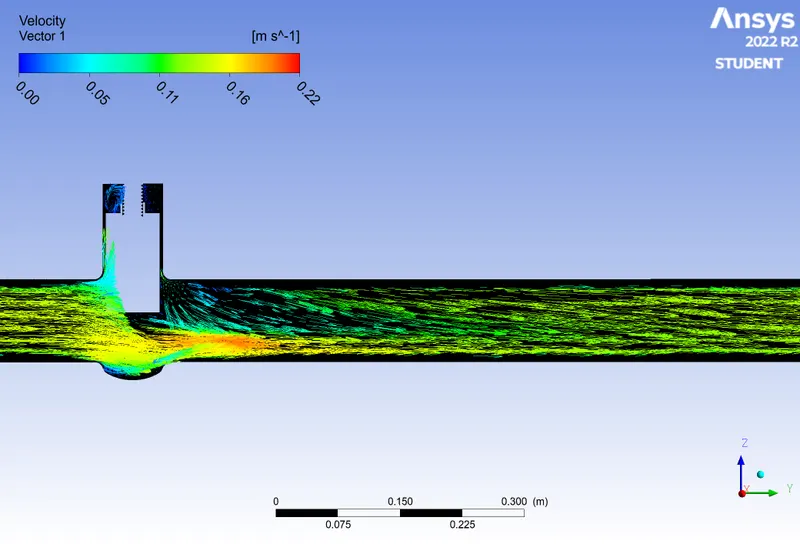
Velocity vector

Animation of streamline

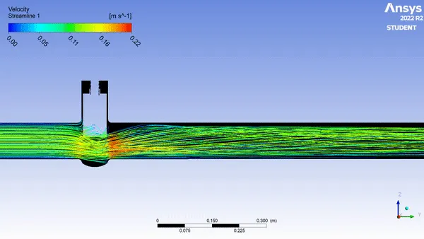
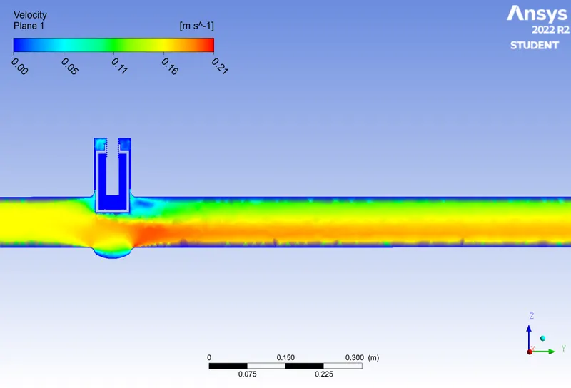
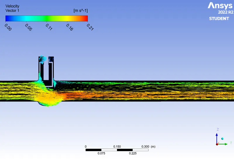
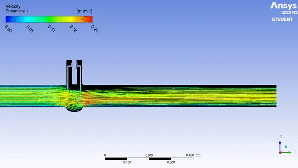
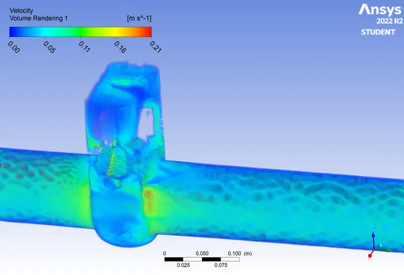
Case 8: Disc position at 80 mm

Velocity contour

Velocity vector

Animation of streamline

Volume render of Velocity for Case 8 : Disc position at 80 mm (For visualizing)

Mass Flow rate at each Design points (cases)

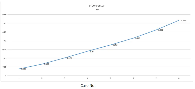
Flow-Factor(kv):

Kv is the flow coefficient in metric units. It is defined as the flow rate in cubic meters per hour [m3/h] of water at a temperature of 16º celsius with a pressure drop across the valve of 1 bar. Cv is the flow coefficient in imperial units.

Flow-coefficient(Cv):

The coefficient of flow (Cv) is a formula which is used to determine a valve's flows under various conditions and to select the correct valve for a flow application. The Cv was designed for use with liquid flows, it expresses the flow in gallons per minute of 60º F water with a pressure drop across the valve of 1 psi.

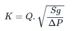
K = Cv , when k is referenced in [gpm] [psi] unit

K = Kv , when k is referenced in [m3/hr] [bar] unit

where Q = mass flow rate

Sg = Specific gravity of water which is equal to 1

DeltaP = Change in pressure or pressure drop across valve

Relation between Kv and Cv:

Cv = Kv*1.156

case	Disc Lift position (mm)	Inlet Pressure (Pa)	Outlet Pressure (Pa)	Pressure Drop (Pa)	Mass Flow rate at Outlet in Kg/s (Leaving)	Mass Flow rate at Outlet in m^3/hr (Leaving)	Flow Coefficient Cv	Flow Factor Kv
1	10	20	0.37	19.63	0.206	0.74	0.046	0.039
2	20	20	0.965	19.035	0.336	1.21	0.077	0.066
3	30	20	2.155	17.845	0.504	1.81	0.119	0.102
4	40	20	3.703	16.297	0.657	2.37	0.162	0.14
5	50	20	5.261	14.739	0.784	2.82	0.204	0.176
6	60	20	6.939	13.061	0.901	3.24	0.249	0.215
7	70	20	8.757	11.243	1.016	3.66	0.303	0.262
8	80	20	10.771	9.229	1.115	4.01	0.367	0.317

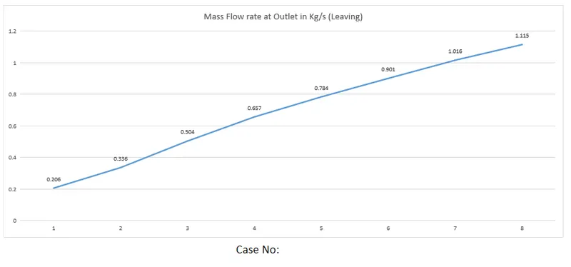
Case no, Vs Mass flow rate graph

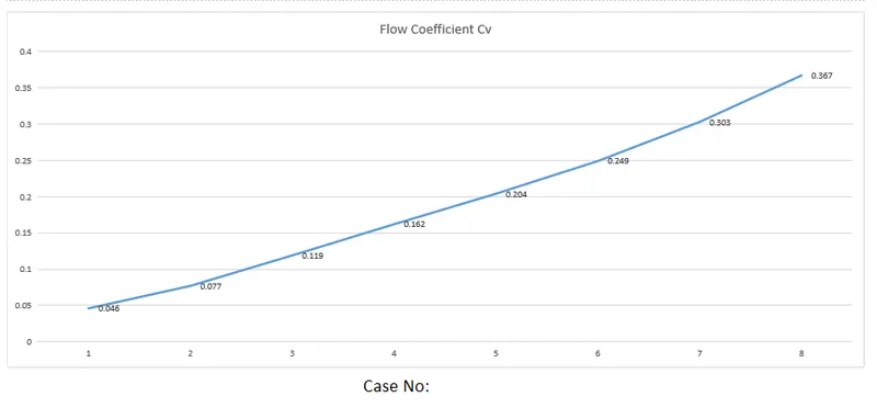
Case no, Vs Flow coeffficient graph

Case no, Vs Flow factor graph

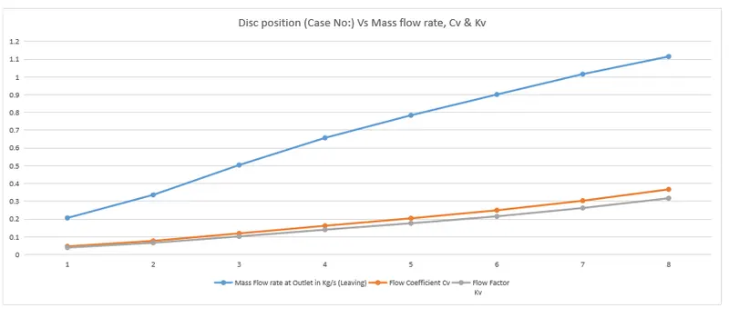
Combined graph for better conclusion

CONCLUSION:

From the above parametric study data and all plots it is very much obvious that as the disc position increases from 10 mm to 80 mm the mass flow rate at the outlet increases. Also, the flow factor values and the flow coefficient values concur the same.

Interesting thing is the venturi effect at the disc for every step increase case by case is giving rise to increased velocity in cases 0.18 to 0.28 m/s and drops to 0.22 m/s in 80 mm open condition.

Since the max velocity occurs at the disc exit radius zone (from velocity contour) that area is prone to surface abrasion in long term, so the material used plays a major role in determining the life of the valve. Say, we can use gun metal valve in place of cast iron valves for high pressure inlet conditions.

INFERENCES:

• As the disc opens more, more mass flow rate at outlet (very obvious).
• Velocity at the disc exit increases and decreses case by case due to venturi effect.
• Total pressure at outlet increases proportional to the disc lift position in case by case.
• Use of parametric study is much of use without having to open the fluent for each case.
• Updating the volume in spaceclaim by context is very much important for smooth operation of solution.

Reference:

https://www.sciencedirect.com/topics/engineering/gate-valve