Week 9 - Parametric study on Gate valve.

CHALLENGE - 9: Parametric Study on Gate Valve

AIM:

To perform a parametric study on the gate valve simulation by setting the opening from 10 % to 80% by using ANSYS FLUENT and to mass flow rates at the outlet for each design point.

OBJECTIVE:

1. To perform a parametric study on the gate valve simulation by setting the opening from 10 % to 80%.
2. To calculate mass flow rates at the outlet for each design points.
3. To calculate the flow coefficient and flow factor for each opening and plot the graph.

THEORY:

• The flow coefficient of a device is a relative measure of its efficiency at allowing fluidflow. It describes the relationship between the pressure drop across a valve or other assembly and the corresponding flow rate
• The use of the flow coefficient offers a standard method of comparing valve capacities and sizing valves for specific applications that is widely accepted by industry.

Mathematically flow factor is represented as

`Kv = Qsqrt((SG)/(DeltaP))`

where

K_v is the flow factor (expressed in m³·h⁻¹).

Q is the flowrate (expressed in cubic metres per hour m³·h⁻¹).

SG is the specific gravity of the fluid (for water = 1).

∆P is the differential pressure across the device (expressed in bar).

Flow coefficient can be calculated from flow factor using the equation

`Cv = (Kv)/0.865`

PROCEDURE:

1. Open ANSYS Workbench 2022R2 select Fluid Flow (Fluent) from Toolbox.

2. Rename the file and left click Geometry and select New Spaceclaim Geometry.

3. Open the geometry STEP or SLDPRT of the geometry in spaceclaim.

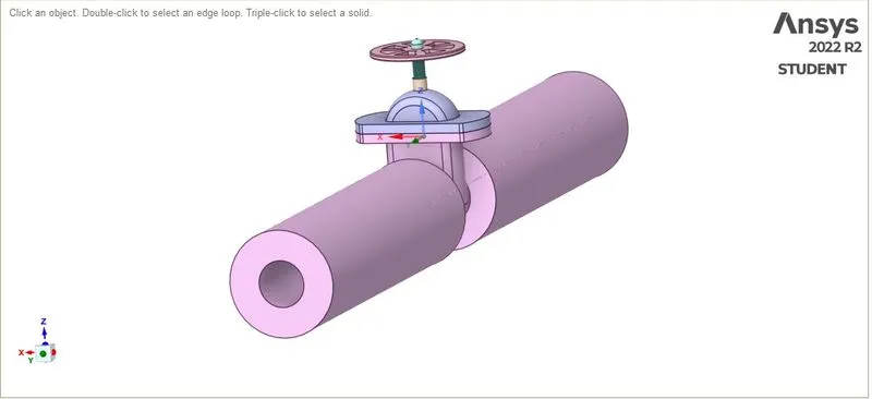
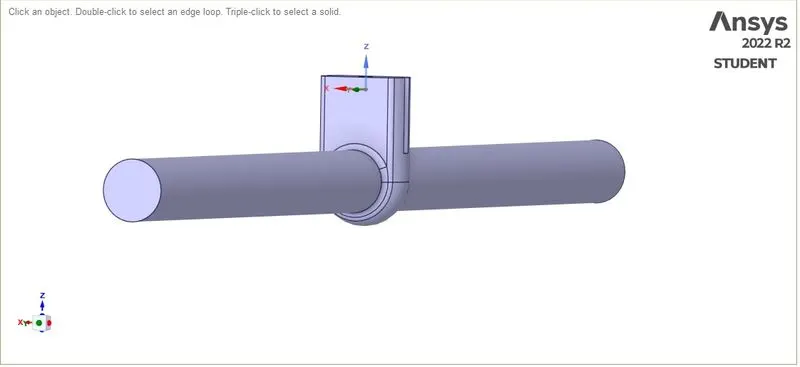
4. Now move the disc by 10 mm and select the create group option from the tree to set the parametric option. Extract the fluid volume by selecting Extract Volume option from Prepare menu on top bar. Then select the edges and click the tick mark now a new volume is created and which can be visible on tree. Now suppress the geometry by selecting the suppress from physics option which helps to provide only the extracted volume for the analysis.

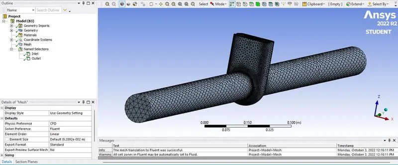
5. Close SpaceClaim and double click on Mesh. Meshing window will appear. Mark Inlet and Outlet on geometry by right clicking each part and selecting Create Name Selection. Now select the mesh from the tree and generate mesh with an appropriate element size (10 mm). The figure shown below represent the geometry after meshing.

6. Close Meshing and double click on Setup, select Double Precision and Fluent window will open. Check all the values and make necessary correction if needed.

7. Select appropriate conditions mentioned below.

Solver - Pressure Based

Gravity - Enabled , Z = -9.81 m/s2

Viscous - k-epsilon model, Realizable with scalable wall function.

Materials - Fluid, Water

Inlet - Pressure Inlet, Pressure = 10 Pa (gaugue pressure)

Outlet - Pressure Outlet , Pressure = 0 Pa (gaugue pressure)

(Assumption: Outlet pressure is considered as atmospheric pressure)

Define surface report with area weighted average of pressure at inlet and outlets and flux report for mass flow rate at outlet for both the cases select output parameters.

Create a longitudinal plane and then create velocity contour on the plane.

Solution Initialization - Standard Initialization.

8. After assigning all the factors click on Run Calculation and set number of iteration and calculate.

9. Now close ANSYS FLUENT, open Parameters present on the workbench, then create design points and update the the design points to obtain the inlet and output pressure and outlet mass flow rate.

The results obtained are shown in the next session.

RESULTS AND DISCUSSION:

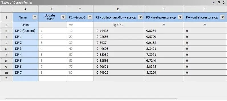
• The figure shown below represents the results obtained for different design points.

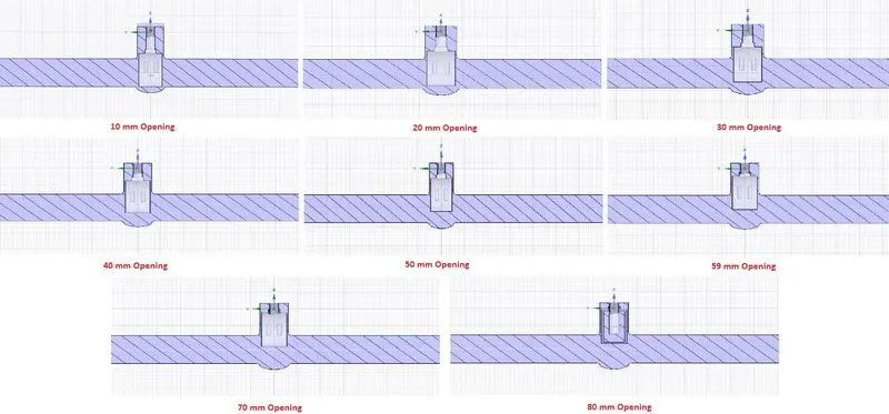
• Position of the valve corresponding to design points (different valve opening) are shown below.

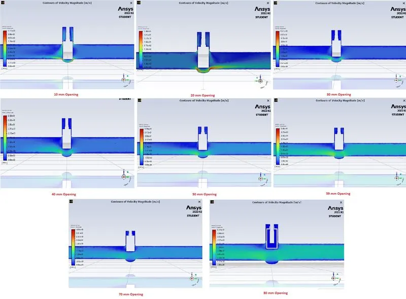
• Velocity contours corresponding to design points (different valve opening) are shown below.

• Calculated flow factors and flow coefficients corresponding to design points (different valve opening) are shown below.

Name	P1 - Group1	P2 - outlet-mass-flow-rate	Flow rate	P3 - inlet-pressure	P4 - outlet-pressure	Flow factor	Flow Coefficient
Units	mm	kg s^-1	m3/h	Bar	Bar	m3/h	m3/h
DP 0	10	-0.14407905	0.51868458	9.82641E-05	0	52.3246058	60.49087375
DP 1	20	-0.22656154	0.815621544	9.57088E-05	0	83.370588	96.38218264
DP 2	30	-0.34369757	1.237311252	9.01818E-05	0	130.29255	150.6272249
DP 3	40	-0.4469559	1.60904124	8.34214E-05	0	176.168538	203.6630495
DP 4	50	-0.55081629	1.982938644	7.39711E-05	0	230.556945	266.5398207
DP 5	59	-0.62586223	2.253104028	6.72491E-05	0	274.750211	317.6303019
DP 6	70	-0.70600504	2.541618144	5.83747E-05	0	332.657971	384.5756889
DP 7	80	-0.74922074	2.697194664	5.32244E-05	0	369.706266	427.4060874

• The plot shown below represents the variation of flow coefficient and flow factors with mass flow rate for different valve openings.

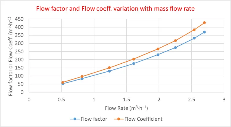
From the above table and figures it is evident that with increase in valve opening mass flow rate increases which further causes the increase in flow factor and flow coefficient. The negative sign in mass flow rate represents the mass is flowing out from outlet.

CONCLUSION:

Parametric study on the gate valve simulation by setting the opening from 10 % to 80% have been carried out by using ANSYS FLUENT. From the simulation it is concluded that with increase in valve opening mass flow rate increases which further causes the increase in flow factor and flow coefficient. Plots, contours and table of the simulation is also reported.