Week 3 - Solving second order ODEs

CHALLENGE - 6 : Solving Second Order ODE (Simple Pendulum)

AIM:

To write program in Matlab that will simulate the pendulum motion by soving the seocond order ODE.

OBJECTIVES:

1. To solve the second order ODE by using ode45 pre-defined function.
2. To plot the variation of displacement and velocity with time (0 - 20 sec).
3. To prepare the animation of motion of the pendulum.

THEORY:

A simple pendulum consists of a ball of mass m hanging on a string of length fixed at one of its end. When the mass is diplaced to an inital angle pendulum swings back and forth in a periodic motion.

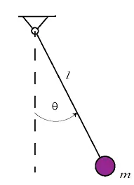
The above figure shows the represntation of pendulum

GOVERNING EQUATION AND EQUATIONS:

The governing equation for the periodic motion of a simple pendulum is given by:

`(d^2 theta)/dt^2+b/m**(d theta)/dt+g/l**sintheta = 0` ------------------------------(1)

where

g = gravity in `m/s^2`,

L = length of the pendulum in `m`,

m = mass of the ball in `kg`,

b=damping coefficient.

As ode45 solver in matlab is for the first order differential equation we need to split this second order differential equation to 2 first order differential equation for that consider.

`theta = theta 1`

`=>(d theta)/dt=(d theta 1)/dt=theta2`

`=>(d^2theta)/dt^2=(d^2theta 1)/dt^2=(d theta2)/dt`

`(1)=> (d theta2)/dt+b/mtheta2+g/lsintheta1`

thus we can write the equation into

1. `=> (d theta2)/dt= -b/mtheta2-g/lsintheta1`
2. `=> (d theta1)/dt=theta2`

`=> d/dt[[theta1],[theta2]] =[[theta2],[-b/mtheta2-g/lsintheta1]]`

Thus second order ODE is splitted into two first order ODEs then it is solved by using Matlab.

Equation to calculate the position of pendulum

1. Fixed point `=> X0 = 0` & `Y0 = 0`
2. Free point `=> X1 = l**sintheta` & ` `Y1 = -l**costheta`

where negative in Y1 represents that pendulum is downward and its on negative y- axis

PROCEDURE:

1. Program is started by using the general commands clear all, close all and clc to clear and close all the pre-occupied operations of Matlab.
2. Provide the input coditions, initial condition and time span till which the program need solve as mentioned in the question.
3. Call the ode 45 function with its syntax ode45(@(t,theta) ode_func(t, theta, ....),t_span,theta_0) where t and theta are the independent and dependent variables of the ODE. Inside the function name provide the input parameter and followed by time span and initial conditions.
4. Define the function ode_func in the new file and save the file with same function name in same folder where the main program is saved.
5. Calculate the dtheta_1 and dtheta_2 as represented in the governing equation and return these values.
6. After calling the function displacement and velocity for 20 sec is stored to results.
7. Plot these velocity and displacement with respect to time.
8. Provide title, axis labels and legends to the plot.
9. To generate the animation start a for loop from i =1 till the length of the results (here we divide the time span to 500 steps).
10. Fix one end of pendulum and other end by using the equation mentioned above.
11. Plot the base line and plot the string of pendulum by starting and end poiints.
12. Plot the ball by using the marker at the free end.
13. Give axis label and title to the plot.
14. Each frame during the iteration is stored to a new array called M, increment ct and end the loops.
15. Create an animation of stored frame by using movie command.
16. Create a video file, open the file, write the file with datas from the array M and close the opened file.
17. Save and Run the file.

The main program which is created on Matlab is attached below.

% Program to solve the ODE represents the equation of motion of 
% simple pendulam followed by plotting the displacement and veloicity and 
% doing an animation of motion.
close all
clear all
clc

% Input condition as per the question
b = 0.05;    % Damping coefficient
g = 9.81;    % Acceleration due to gravity (m/s^2)
l = 1;       % Length of pendulam (m)
m = 1;       % Mass of pendulam (kg) 

% Initial Condition
theta_0 = [0;3];      % Dispacement = 0 and velocity = 3m/s at t = 0.

t_span = linspace(0,20,500);  % Time span of 20 s

% Calling the ode45 fuction with its general syntax by a function name called ode_func.
[t,results] = ode45(@(t,theta) ode_func(t, theta, b,g,l,m),t_span,theta_0);

% Plotting the displacement and velocity variation
figure(1)
plot(t, results(:,1));         % Plotting displacement
hold on
plot(t, results(:,2));         % Plotting velocity

% Giving Label, Title and Legend to the plot
ylabel('Dispalcement and Velocity');
xlabel('Time (s)');
title('Variation of dispacement and velocity with time');
legend('Displacement','Velocity');
hold off

% Generating animation of simple pendulam
ct = 1;
figure(2)                      % Saving to figure 2

% Defining the for loop for animation
for i=1:length(results(:,1))   

    % Fixing one end of pendulam
    x_0 = 0;                  
    y_0 = 0;

    % Calculating the motion of pendulam 
    x_1 = l*sin(results(i,1));
    y_1 = -l*cos(results(i,1)); % Negative to represent the pendulam is on negative y- axis
    
    plot([-2 2], [0 0])         % Ploting a base line
    hold on
    
    % Ploting the string of pendulam
    plot([x_0 x_1], [y_0 y_1], 'LineWidth', 2,'Color','b')
    axis([-2 2 -2 2]);          % Setting the axis         

    % Plotting the ball at the end by using a 'O' Marker
    plot(x_1, y_1, 'O', 'Markersize',20, 'Color', 'r')
    
    % Giving Label and Title to the plot
    ylabel('Y-Axis');
    xlabel('X-Axis');
    title('Motion of simple pendulam');
    
    pause(0.03)
    M(ct) = getframe(gcf);     % Stroing each frame to an array called M.
    hold off
    ct = ct + 1;                % Incrementing the ct.
end

movie(M);      % Creating a animation by using movie command and array M.

% Creating a video file in the computer folder.
videofile = VideoWriter('Simple Pendulam.avi','Uncompressed AVI'); 

open(videofile);  % Opening the video file.

writeVideo(videofile,M);  % Writing the video file.

close(videofile);  % Closing the video file.

The ode_func function script used for the program is attached below.

% Defining the fuction ode_fun to return the theeta value
function [dtheta_t] = ode_func(t,theta,b,g,l,m)

% Writing the second order ODE to two first order ODEs, theta1 and theta2.
theta1 = theta(1);
theta2 = theta(2);

% Solving the two first order ODEs/
dtheta1_dt = theta2;
dtheta2_dt = -(b/m)*theta2-(g/l)*sin(theta1);

% Storing it to dtheta_t
dtheta_t = [dtheta1_dt;dtheta2_dt];
end

RESULTS:

The figure attached below shows the plot of variation of displacement and velocity with time.

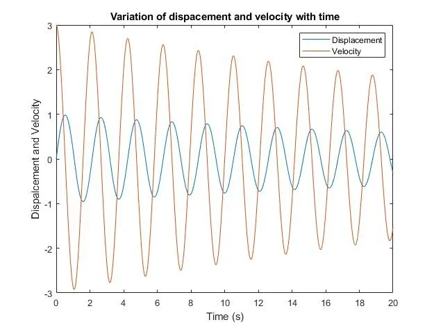
Here we can see initially displacement is 0 but when a velocity of 3 m/s is applied it starts to oscillate. That is we can say at t = 0 `theta`= 0 and velocity = 3 m/s. Then from the next time step onwards velocity decreases but `theta` varies. The animation of motion is attached to the google drive and link is provided below.

https://drive.google.com/file/d/1a8zh-L1YnUAWW6qf9p0WxghQbhCbuT6Y/view?usp=sharing

Errors encountered.

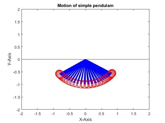
During the execution of the program there were no syntax errors , But a logical error was there, while creating the animation forogot to mention hold off comand and which leads to the following output figure.

CONCLUSION:

A program to solve the second order ODE by using ode45 function is carried out by using Matlab and for the same motion of simple pendulum is considered . During the study a plot of variation of velocity and displacement with time as well as the motion of the pendulum were also carried out.