Project 2 - Rankine cycle Simulator

PROJECT - 2: Rankine Cycle Simulator

AIM:

To study the fundamentals of Rankine cycle and to write a Matlab program to create rankine cycle simulator.

OBJECTIVE:

1. To understand the basics of Rankine Cycle
2. To create a Matlab program for rankine cycle simulator the program should plot both T-s and h-s diagram, should display the state point conditions, the thermal efficiency and the Back Work Ratio (BWR) based on the values provided by the user.

THEROY:

Rankine cycle is the idealized thermodynamic cycle which describes the working of a typical steam power plant. The layout of a typical rankine cycle is shown below.

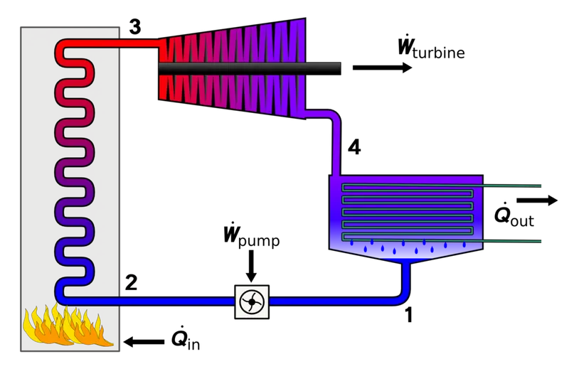
A typical rankine cycle mainly consist of

1. Pump
2. Boiler
3. Turbine
4. Condenser.

T - S diagram of the same is shown below

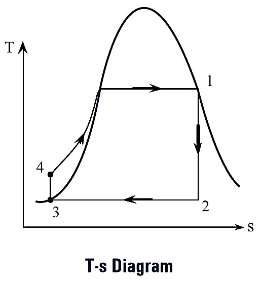
Ranline cycle operates in mainly four process

Process 1 - 2: Adiabatic expansion in turbine

Process 2 - 3: Constant pressure heat rejection in condenser

Process 3 - 4: Adiabatic increase in pressure in pump

Process 4 - 1: Constant pressure heat addition in boiler

Rankine cycle simulator is simulation alogirthm which is used to find out all the state points of the cycle, to plot T-s and h-s diagram of the cycle, to find the net work output, thermal efficiency, back wok ratio of the cycle based upon the input values provided by the user. In this case Turbine inlet and outlet pressure and turbine inlet temperature is considered as the input to the simulator.

For solving the problem a function scrpit called XSteam is used to extract the values of different thermodynamic data of water and steam at different conditions.

GOVERNING EQUATIONS AND FORMULAS USED

The main equations which are considered during coding shown below

Process 1 - 2: Adiabatic expansion in turbine

s1 = s2 (entrpoy remains same as the process is adiabatic)

dryness fraction `x2 = ("s"2 - "sf2")/("sg2"- "sf2")`

`"h2" = "hf2"+("x2"**("hg2"-"hf2"))`

Turbine work Wt = h1 -h2

Process 2 - 3: Constant pressure heat rejection in condenser

p2 = p3

Heat rejected, Q_out = h2 - h3

Process 3 - 4: Adiabatic increase in pressure in pump

s3 = s4

Pump work, Wp = h4 - h1

Process 4 - 1: Constant pressure heat addition in boiler

p1 = p4

Heat addition, Q_in = h1 - h4

Net work, W_net = Wt + Wp

Thermal Efficiency, `eta = ("W_net")/("Q_in")`

Work Ratio `"WR" = ("W_net")/("Wt")`

BWR = 1-WR

PROCEDURE

1. Program is started by using the general commands clear all, close all and clc to clear and close all the pre-occupied operations of Matlab.
2. Provide the input conditions such as turbine inlet temperature and pressure and turbine outlet pressure by using input command.
3. Calling the fuction XSteam to get different state points properties like Temperature(T), Pressure(p)m Enthalpy(h) and Entropy(s) by using the concept used above in the governing equation.
4. After extracting the 4 state point extract 2 more state points 5 and 6 on the saturated liquid line and saturated vapour line in the process 4-1 to create the dome for T-s and h-s plot.
5. Create a temperature array and find the enthalpy and entropy value corresponding to the temperature array using a for loop to plot dome of t-s and h-s diagram.
6. Plot the T-s and h-s diagram initially by plotting the stae points and then joining the points also create the SVL and SLL.
7. Calculate thermal efficiency, net work, work ratio and back work ratio by using the equation mentioned above.
8. Print all the state point condition and resulted output.
9. Save and run the program.

% Program to create a Rankine Cycle Simulator
close all 
clear all
clc

% Input conditions by user

% Turbine Inlet 
t1 = input('Enter the Temperature(in deg C) of turbine inlet: ');
p1 = input('Enter Pressure(bar) of turbine inlet: ');

% Turbine Outlet
p2 = input('Enter Pressure(bar) of turbine outlet: ');

% Properties at different state points by using function XSteam

% Turbine Inlet or Boiler Outlet (State Point- 1)
h1 = XSteam('h_pT',p1,t1);
s1 = XSteam('s_pT',p1,t1);

% Turbine Outlet or Condenser Inlet (State Point- 2)
s2 = s1;                    % Adiabatic Expansion      
t2 = XSteam('Tsat_p',p2); 
sf2 = XSteam('sL_p',p2);
sg2 = XSteam('sV_p',p2);
hf2 = XSteam('hL_p',p2);
hg2 = XSteam('hV_p',p2);
x2 = ((s2-sf2)/(sg2-sf2));  % Dryness fraction calculation
h2 = (hf2 + x2*(hg2 - hf2));

% Condenser Outlet or Pump Inlet (State Point- 3)
p3 = p2;    % Constant pressure heat rejection
t3 = t2;    % Phase changer temperature remain constant.
hf3 = hf2;
sf3 = sf2;
h3 = hf3;
s3 = sf3;

% Pump Outlet or Boiler Input (State Point -4)
s4 = s3;  % Adiabatic increase in pressure or compression
p4 = p1;  % Constant pressure heat addition
h4 = XSteam('h_ps',p4,s4);
t4 = XSteam('T_ps',p4,s4);

% Defining state point on the Saturated liquid and vapour line (State point - 5 & 6)
p5 = p1;                       % Constant Pressure heat addition
t5 = XSteam('Tsat_p',p5);
h5 = XSteam('hL_p',p5);
s5 = XSteam('sL_p',p5);

p6 = p1;                       % Constant Pressure heat addition
t6 = t5;                       % Phase change temperature remains constant
h6 = XSteam('hV_p',p6);
s6 = XSteam('sV_p',p6);

% Defining saturated liquid and saturated vapour line
t = linspace(0,t1,t1);
for i = 1:t1                         % for loop to create SLL and SVL
    hl(i) = XSteam('hL_T',t(i));
    sl(i) = XSteam('sL_T',t(i));
    hg(i) = XSteam('hV_T',t(i));
    sg(i) = XSteam('sV_T',t(i));
end

% Plotting T-S diagram
figure(1)
hold on

% Defining all the state points 
plot(s1,t1,'*','color','g')            
text(s1,t1,'1','color','r')
plot(s2,t2,'*','color','g')
text(s2,t2,'2','color','r')
plot(s3,t3,'*','color','g')
text(s3,t3,'3','color','r')
plot(s4,t4,'*','color','g')
text(s4,t4,'4','color','r')

% Creating the plot using the defined state points
plot([s1 s2],[t1 t2], 'LineWidth',2, 'color','k')
plot([s2 s3],[t2 t3], 'LineWidth',2, 'color','k')
plot([s3 s4],[t3 t4], 'LineWidth',2, 'color','k')
plot([s4 s5],[t4 t5], 'LineWidth',2, 'color','k')
plot([s5 s6],[t5 t6], 'LineWidth',2, 'color','k')
plot([s6 s1],[t6 t1], 'LineWidth',2, 'color','k')

% Creating the SLL and SVL
plot([sl sg], [t t], 'LineWidth',2, 'Color','r')

% Title, Label and Legends to the plot
xlabel('Entropy (S)')
ylabel('Temperature (T)')
title('T-S Diagram of Rankine Cycle')
legend('State Points')
saveas(figure(1), 'T-S Diagram.jpg')      % Saving the figure.

figure(2)
hold on

% Defining all the state points
plot(s1,h1,'*','color','g')
text(s1,h1,'1','color','r')
plot(s2,h2,'*','color','g')
text(s2,h2,'2','color','r')
plot(s3,h3,'*','color','g')
text(s3,h3,'3','color','r')
plot(s4,h4,'*','color','g')
text(s4,h4,'4','color','r')

% Creating the plot using the defined state points
plot([s1 s2],[h1 h2], 'LineWidth',2, 'color','k')
plot([s2 s3],[h2 h3], 'LineWidth',2, 'color','k')
plot([s3 s4],[h3 h4], 'LineWidth',2, 'color','k')
plot([s4 s5],[h4 h5], 'LineWidth',2, 'color','k')
plot([s5 s6],[h5 h6], 'LineWidth',2, 'color','k')
plot([s6 s1],[h6 h1], 'LineWidth',2, 'color','k')

% Creating the SLL and SVL
plot([sl sg], [hl hg], 'LineWidth',2, 'Color','r')

% Title, Label and Legends to the plot
xlabel('Entropy (S)')
ylabel('Enthalpy (H)')
title('H-S Diagram of Rankine Cycle')
legend('State Points')
saveas(figure(2), 'H-S Diagram.jpg')      % Saving the figure.


wt = h1-h2;               % Turbine work output
wp = h4-h3;               % Pump work input
w_net = wt - wp;          % Net work
  
q_in = h1 - h4;           % Heat input
q_out = h2-h3;            % Heat rejected
eff = (w_net/q_in)*100;   % Thermal Efficiency

WR = w_net/wt;            % Work Ratio
BWR = 1 - WR;             % Back Work Ratio

% Printing the results
fprintf('\n State Point-1 \n Temperature T1 %f deg C \n Pressure P1 %f bar \n Enthalpy H1 %f kJ/kg \n Entropy S1 is %f \n',t1,p1,h1,s1)
fprintf('State Point-2 \n Temperature T2 %f deg C \n Pressure P2 %f bar \n Enthalpy H2 %f kJ/kg \n Entropy S2 is %f \n',t2,p2,h2,s2)
fprintf('State Point-3 \n Temperature T3 %f deg C \n Pressure P3 %f bar \n Enthalpy H3 %f kJ/kg \n Entropy S3 is %f \n',t3,p3,h3,s3)
fprintf('State Point-4 \n Temperature T4 %f deg C \n Pressure P4 %f bar \n Enthalpy H4 %f kJ/kg \n Entropy S4 is %f \n',t4,p4,h4,s4)
fprintf('\n Turbine work output(Wt) is %f kJ',wt)
fprintf('\n Pump work input(Wp) is %f kJ',wp)
fprintf('\n Net work (Wnet) is %f kJ',w_net)
fprintf('\n Back Work Ratio (BWR) is %f',BWR);
fprintf('\n Thermal Efficiency of Cycle is %f',eff)

RESULTS:

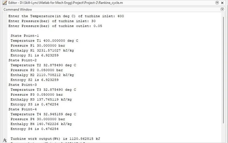
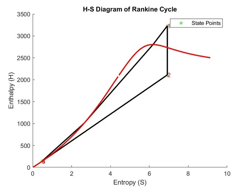
Output obtained after execution the program is shown below here input temperature and pressure of turbine are consdered as 400 deg C and 30 bar and output pressure of turbine is considered as 0.05bar

T-s and h-s diagram obtained for this case are attached below

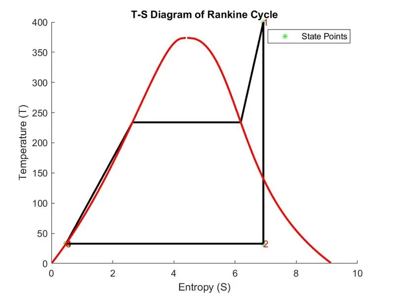
Screenshot of workspace

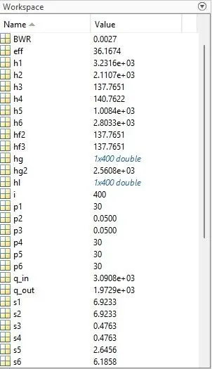
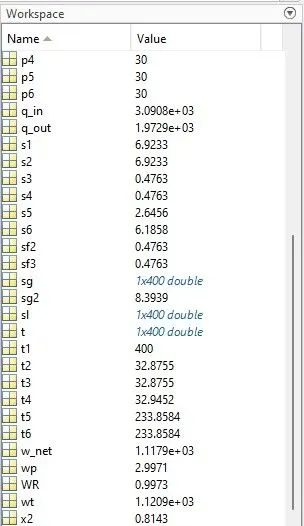
From the simulation it is concluded that for the given case the thermal efficiency of the rankine cycle is 36.16%, Back work ratio(BWR) is 0.00267, Net work(W_net) is 1117.86 kJ.

CONCLUSION:

A Matlab program for rankine cycle simulator is created in Matlab and its thermal efficiecny, net work, back work ratio, T-s and h-s diagram for the given case is calculated and the results are studied.