Week 9 - Parametric study on Gate valve.
Aim
Perform a parametric study on the given valve geometry with openings from 10% to 80% and obtain the mass flow rate and flow coefficient/flow factor for each valve opening.
Introduction
Gate Valves are valves that open by lifting and dropping a barrier that is placed normal to the flow direction. A fully raised gate valve will offer no flow resistance and let the entire flow pass through. A partially closed gate valve will block the flow and let only a percentage of the mass pass through for a given fluid inlet pressure. This percentage of mass flow passing across the gate valve depends on the percentage of pipe that is blocked by the gate valve and needs to be estimated by experimentation or numerical analysis. Flow factor and flow coefficient are parameters that relate the pressure drop across the valve to the volumetric flow rate.
Flow Factor (`K_v`)
Flow factor (`K_v`) is defined as the flow of water with temperature ranging from `5 - 30^circ C` through a valve in cubic meters per hour (m3/h) with a pressure drop of 1 bar and is given by:
`K_v = Q*sqrt((SG)/(Delta P))`
where,
Q - Volumetric Flow Rate [`m^3`/hr]
SG - Specific gravity of the fluid [-]
`Delta P` - Pressure drop across the gate valve [bar]
Flow Coefficient (`C_v`)
Flow Coefficient (`C_v`) is defined as the flow of water with a temperature of `60 ^circ F` through a valve in gallons per minute with a pressure drop of 1 pound per square inch [psi] and is given by:
`C_v = Q*sqrt((SG)/(Delta P))`
where,
Q - Volumetric Flow Rate [GPM]
SG - Specific gravity of the fluid [-]
`Delta P` - Pressure drop across the gate valve [psi]
The relation between `C_v` and `K_v` is given as [1]:
`C_v`= 1.16 `K_v` and
`K_v`= 0.862 `C_v`
Method
Geometry and Fluid Domain
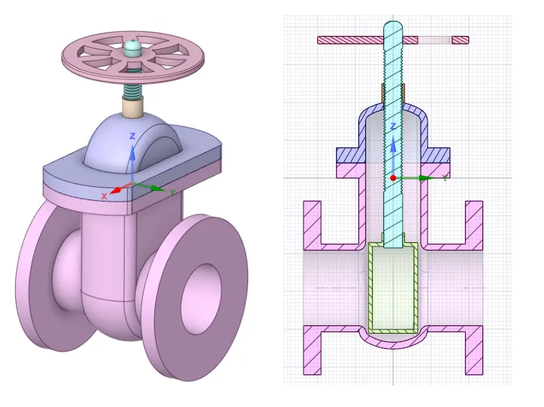
The geometry of the given gate valve along with a cross-sectional view can be seen in the images below. The cross-sectional view shows the gate valve in the fully-closed state.
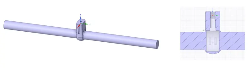
To ease the CFD simulations on the gate valve, the lengths of the piping on either side of the gate valve are pulled to about 800mm while extracting the fluid volume. This will ensure the flow has adequate space to stabilize before and after the gate valve which is crucial to establish a steady state mass flow at the outlet. The resulting fluid volume can be seen in the image below.
Mesh Generation
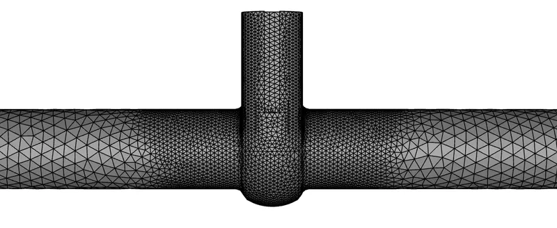
An unstructured tetrahedral mesh was generated over the fluid volume with global max element sizing of 0.02m. A sphere of influence body-sizing was generated at the gate valve with a sphere radius of 0.145m and element sizing of 5.5e-3m. The resulting mesh had roughly 370K cells and was subject to a slight increase or decrease based on the gate valve opening and can be seen below.

Solver and Boundary Conditions
All simulations were performed on ANSYS Fluent 2022 R2. Water at default properties was used as the fluid for the simulations. A pressure inlet boundary condition with a total guage pressure of 10Pa was applied at the inlet and a pressure outlet boundary condition with 0 gauge pressure relative to the atmosphere was applied at the outlet. All walls on the pipe geometry and valve were set to no-slip condition. A gravity of 9.81 m/`s^2` was applied acting in the downwards direction.
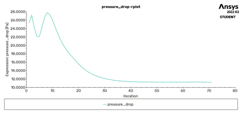
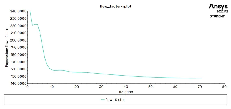
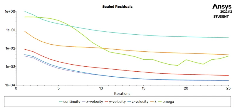
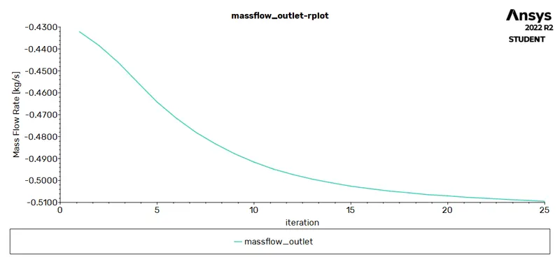
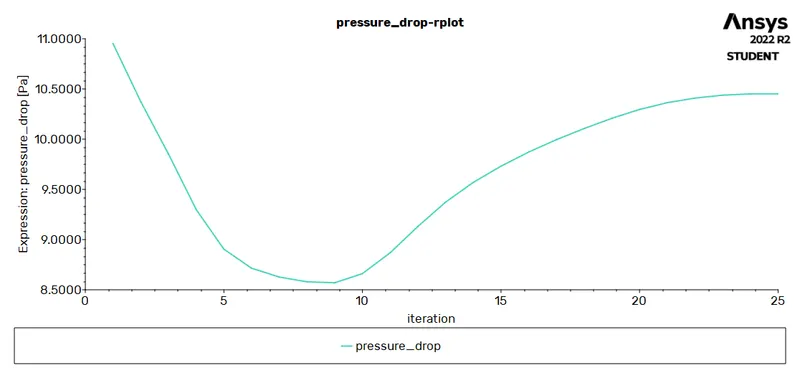
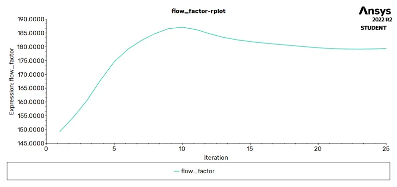
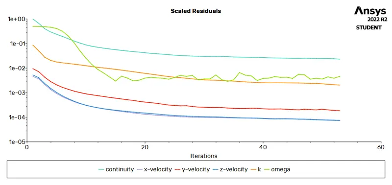
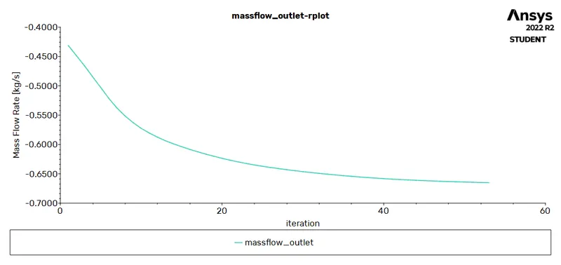
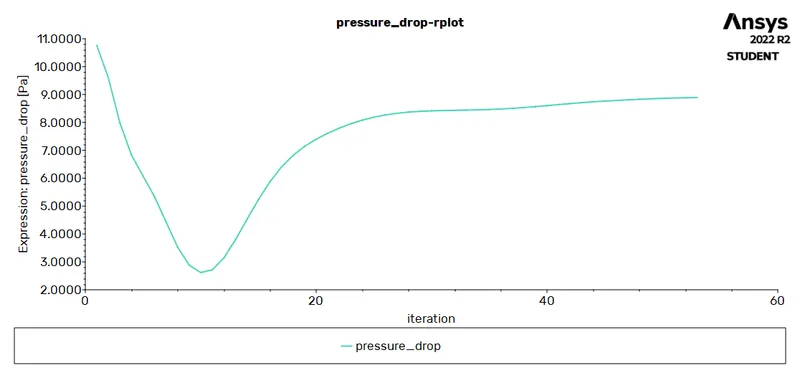
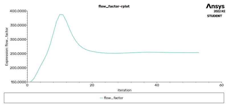
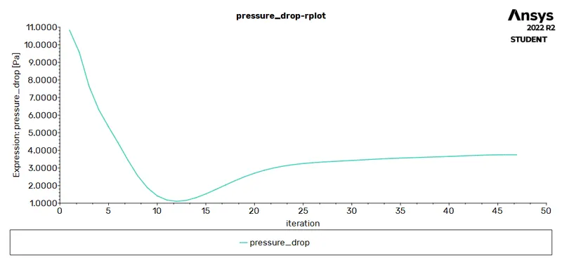
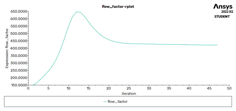
The steady-state pressure-based PV coupled solver was used to discretize the flow parameters. Turbulence in the flow was predicted using the two-equation K-Omega SST model. The second order scheme was used to estimate the pressure, the second order upwind scheme was used to estimate momentum and energy and the first order upwind scheme was used to estimate the turbulence parameters. The solution was initialized by a standard initialization. The simulation was run with pseudo transient time stepping with an automatic global conservative length scale. Convergence was checked by the variations in the pressure drop across the gate valve, the mass flow rate at the outlet and the flow factor not exceeding 1e-3 units across iterations. Simulations typically took 30-100 iterations to achieve convergence.
The image below shows the typical `y^+` on the walls of the fluid volume across each simulation.
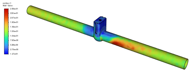
The `y^+` is under 5 in the regions close to the gate valve and increases to a maximum of 25 in the extended regions of the pipe. In Fluent, the K-Omega SST model uses a `y^+` insensitive wall function which switches between resolving the boundary layer and modelling the boundary layer using wall functions based on the `y^+` on that mesh. Resolving the boundary layer is crucial near the gate valve as it is the region of interest in the analysis, the extended regions on the domain can be subjected to a wall functions modelling approach to save up the computational cost of the analysis.
Parametrization of the geometry and solution
The opening of the gate valve was parametrized by moving the valve up the spindle for a specific distance. The diameter of the pipe is 100mm so a 10% valve opening implies a 10mm opening on the valve and so on. Estimations of pressure drop were obtained by using point probes before and after the gate valve. The output parameters for the various design points were mass flow rate at the outlet, pressure drop across the gate valve, and flow factor across the gate valve.
Results
Case 1: 10% Opening - 10mm valve lift
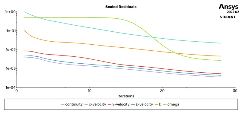
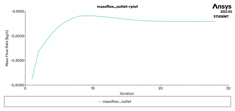
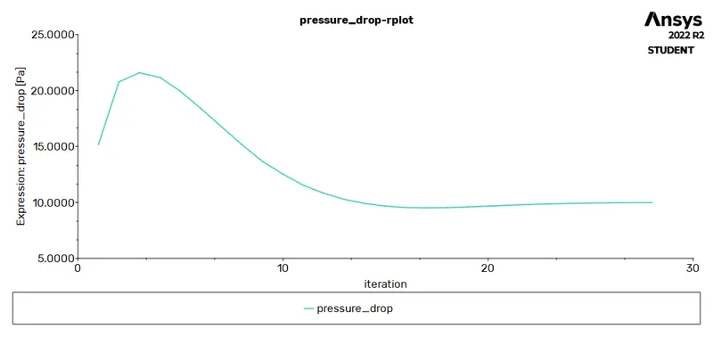
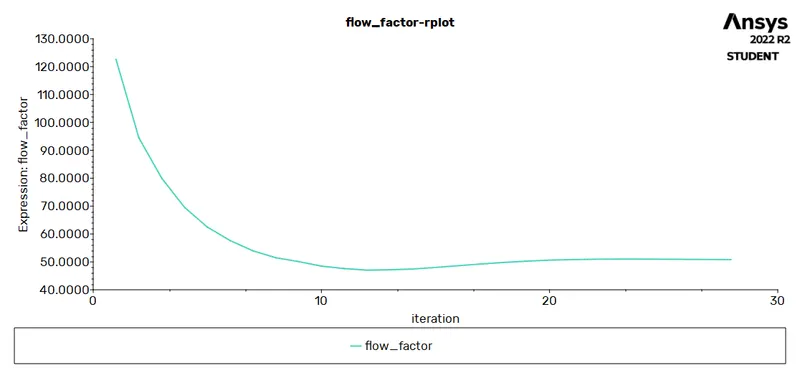
Convergence of the simulation was ensured using the scaled residuals, mass flow at the outlet, pressure drop and flow factor as shown below.
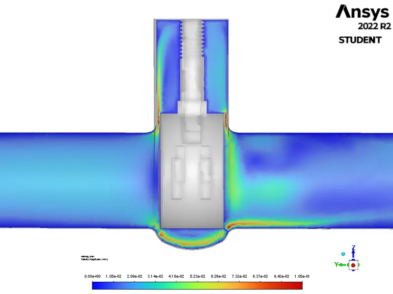
The image below shows the contour of Velocity magnitude at the mid-plane of the pipe.
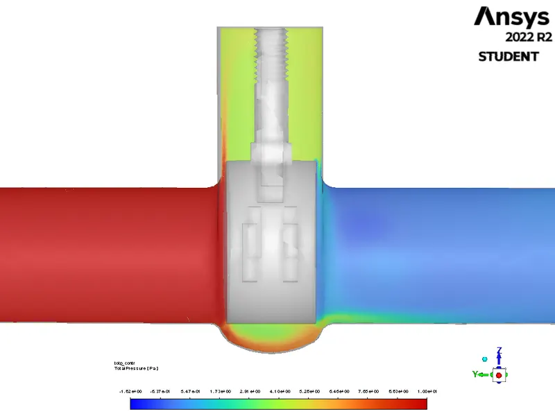
The image below shows the contour of total pressure at the mid-plane of the pipe.
Case 2: 20% Opening - 20mm valve lift
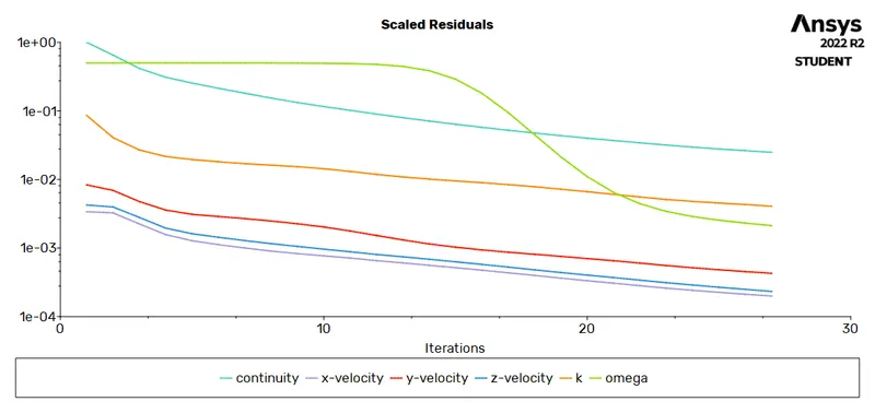
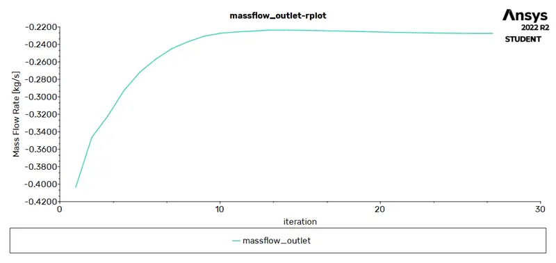
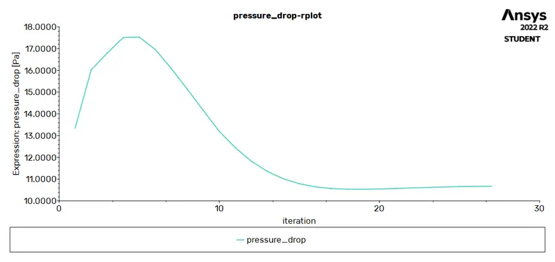
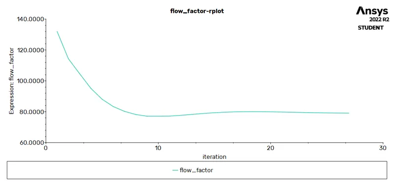
Convergence of the simulation was ensured using the scaled residuals, mass flow at the outlet, pressure drop and flow factor as shown below.
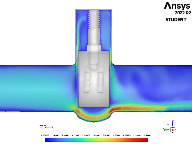
The image below shows the contour of Velocity magnitude at the mid-plane of the pipe.
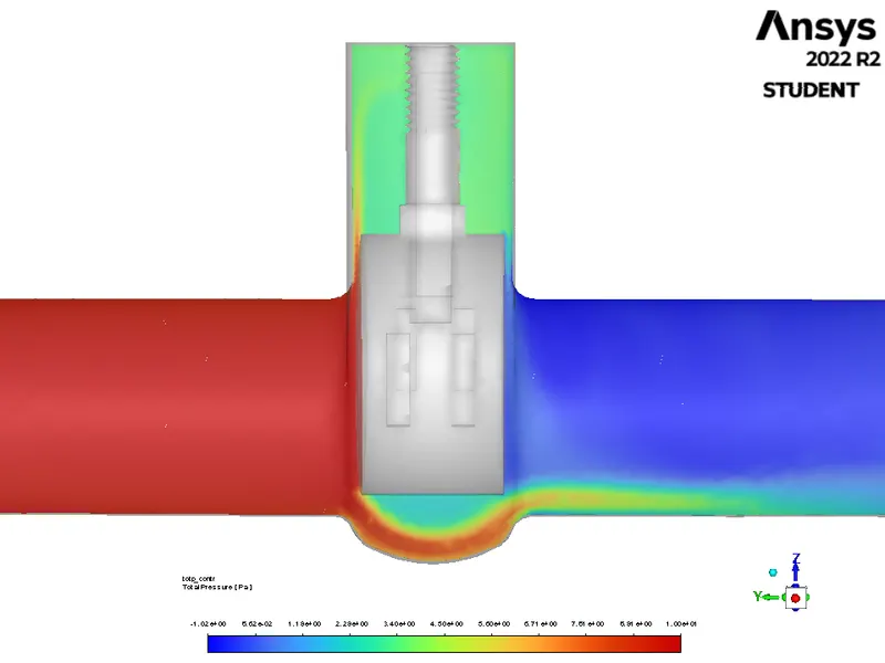
The image below shows the contour of total pressure at the mid-plane of the pipe.
Case 3: 30% Opening - 30mm valve lift
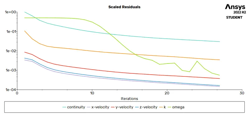
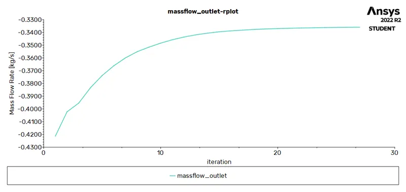
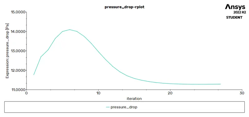
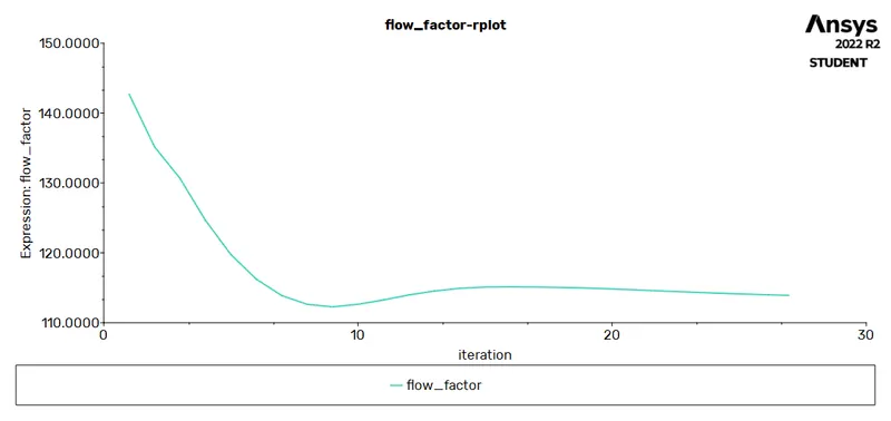
Convergence of the simulation was ensured using the scaled residuals, mass flow at the outlet, pressure drop and flow factor as shown below.
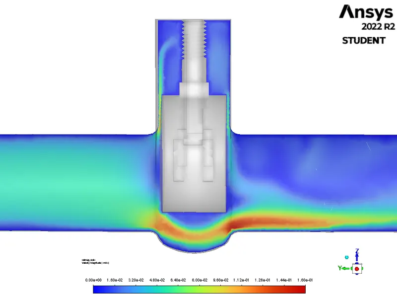
The image below shows the contour of Velocity magnitude at the mid-plane of the pipe.
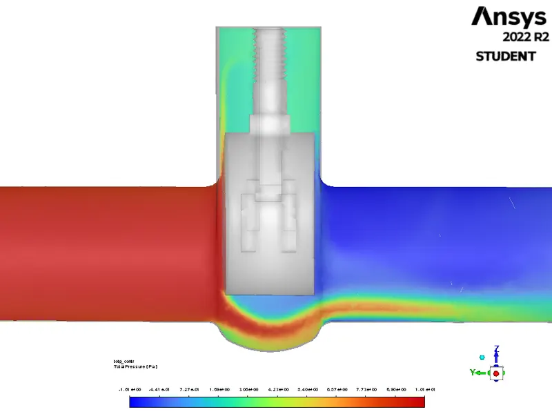
The image below shows the contour of total pressure at the mid-plane of the pipe.
Case 4: 40% Opening - 40mm valve lift
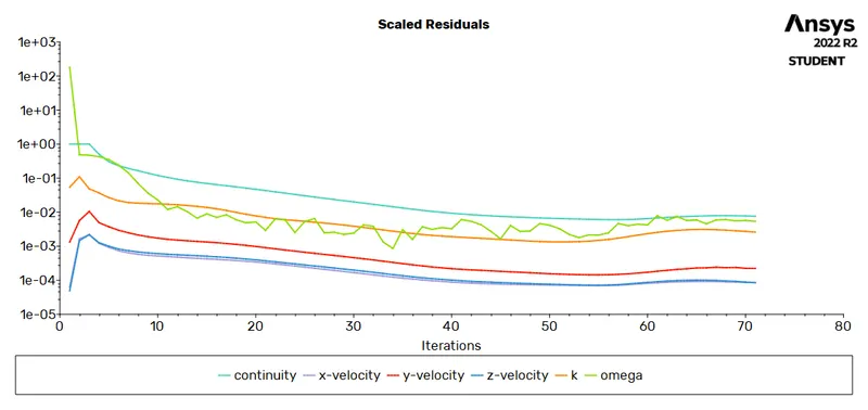
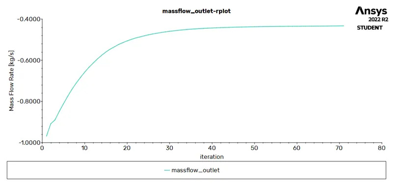
Convergence of the simulation was ensured using the scaled residuals, mass flow at the outlet, pressure drop and flow factor as shown below.
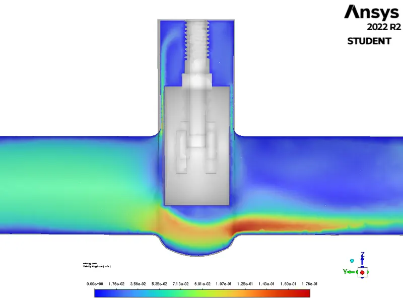
The image below shows the contour of Velocity magnitude at the mid-plane of the pipe.
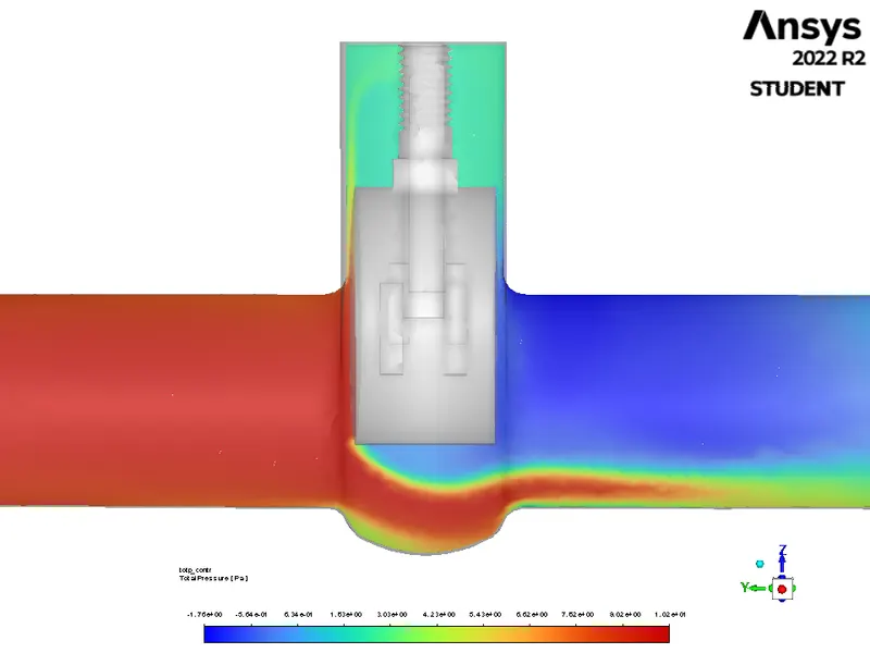
The image below shows the contour of total pressure at the mid-plane of the pipe.
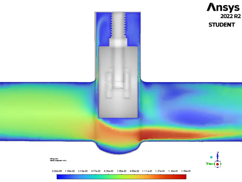
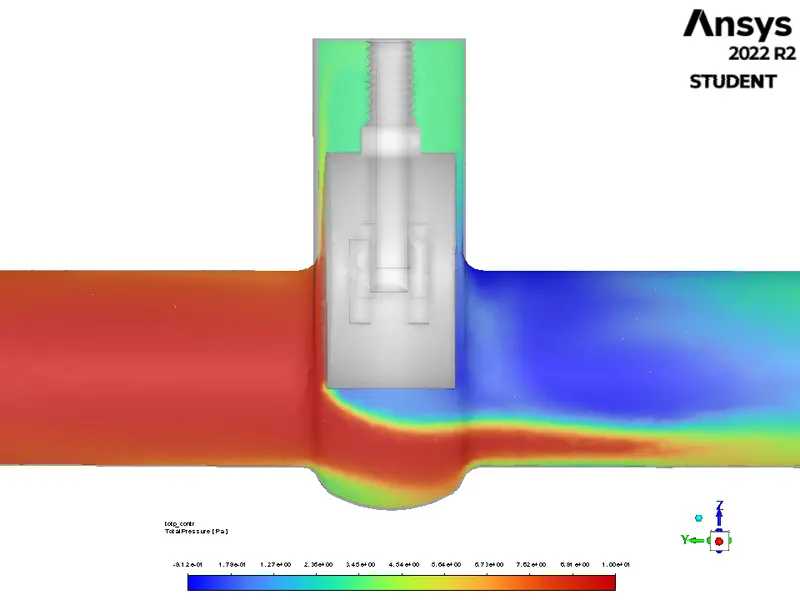
Case 5: 50% Opening - 50mm valve lift
Convergence of the simulation was ensured using the scaled residuals, mass flow at the outlet, pressure drop and flow factor as shown below.
The image below shows the contour of Velocity magnitude at the mid-plane of the pipe.
The image below shows the contour of total pressure at the mid-plane of the pipe.
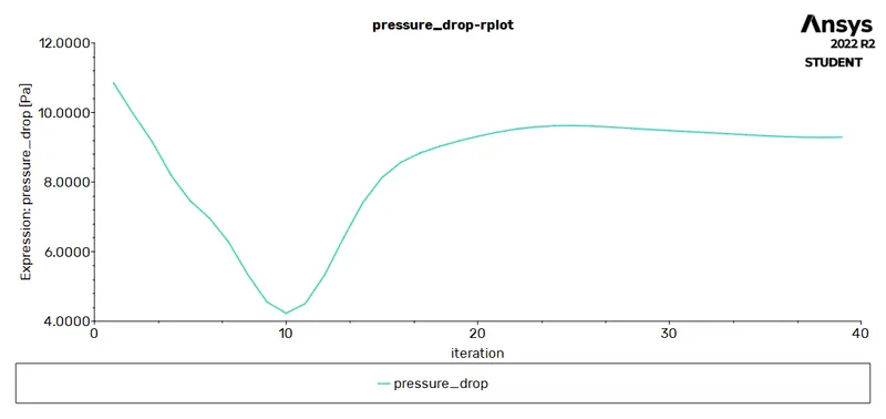
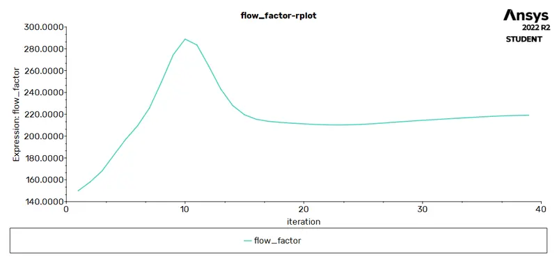
Case 6: 60% Opening - 60mm valve lift
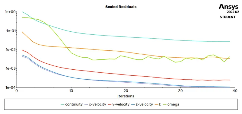
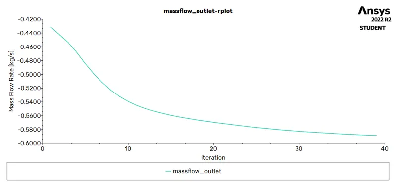
Convergence of the simulation was ensured using the scaled residuals, mass flow at outlet, pressure drop and flow factor as shown below.
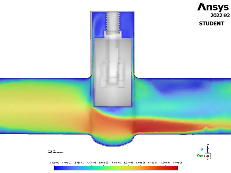
The image below shows the contour of Velocity magnitude at the mid-plane of the pipe.
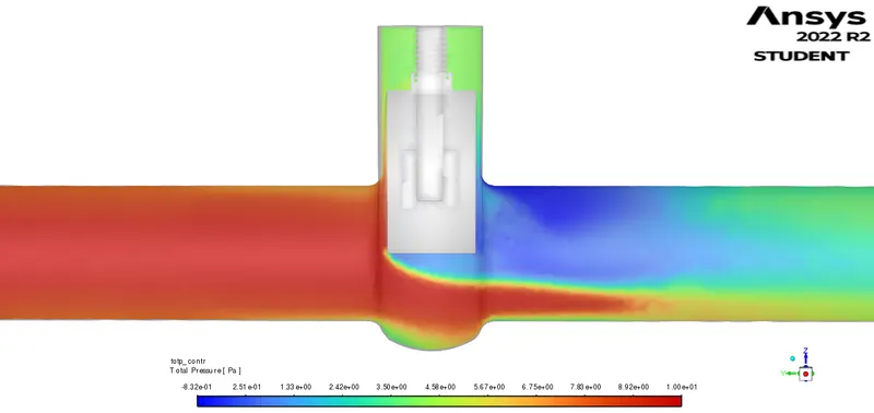
The image below shows the contour of total pressure at the mid-plane of the pipe.
Case 7: 70% Opening - 70mm valve lift
Convergence of the simulation was ensured using the scaled residuals, mass flow at the outlet, pressure drop and flow factor as shown below.
The image below shows the contour of Velocity magnitude at the mid-plane of the pipe.
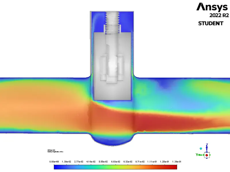
The image below shows the contour of total pressure at the mid-plane of the pipe.
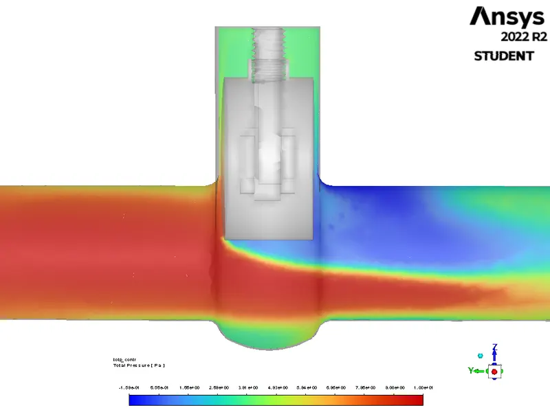
Case 8: 80% Opening - 80mm valve lift
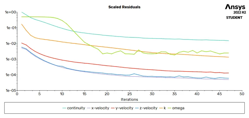
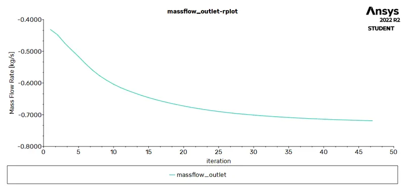
Convergence of the simulation was ensured using the scaled residuals, mass flow at the outlet, pressure drop and flow factor as shown below.
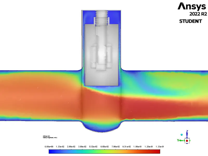
The image below shows the contour of Velocity magnitude at the mid-plane of the pipe.
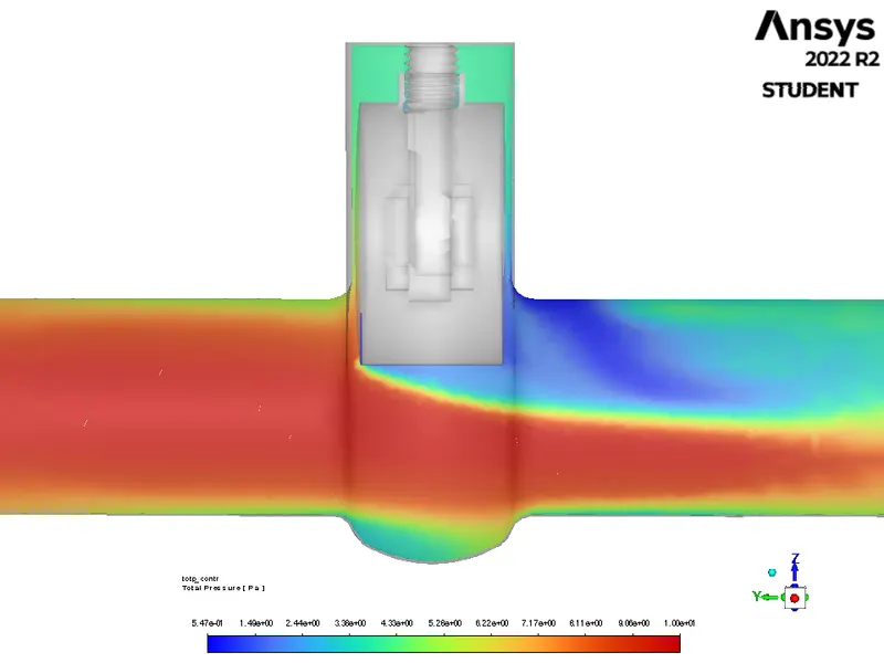
The image below shows the contour of total pressure at the mid-plane of the pipe.
Final Results
The table below shows the mass flow at the outlet, pressure drop across the gate valve and the flow factor.
| Case Id | Valve Opening | Mass Flow Rate at Outlet [kg/s] | Flow Factor [-] | Flow coefficient [-] |
| 1 | 10mm | 0.141 | 50.817 | 58.948 |
| 2 | 20mm | 0.227 | 79.071 | 91.722 |
| 3 | 30mm | 0.336 | 113.9 | 131.128 |
| 4 | 40mm | 0.433 | 147.42 | 171.012 |
| 5 | 50mm | 0.509 | 179.35 | 208.043 |
| 6 | 60mm | 0.589 | 219.12 | 254.176 |
| 7 | 70mm | 0.665 | 253.6 | 294.173 |
| 8 | 80mm | 0.719 | 421.69 | 489.166 |
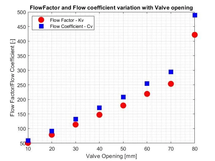
With the opening of the valve, the mass flow rate at the outlet is seen to increase steadily with an increasing flow factor/ flow coefficient. This is due to the decrease in obstruction of the flow by the valve. As the total pressure of the flow is kept constant, there is not enough pressure to push through the gate valve at low valve openings, this leads to a drop in the mass flow rate at the outlet. The flow factor/ flow coefficient has a lower value wherever obstruction of the flow is high and increases as the opening is increased.
The plot below shows the variation of the flow factor and flow coefficient with the valve opening.
Conclusion
A parametric numerical study was performed on the given Gate Valve with valve openings from 10-80% for a specified total gauge pressure of 10Pa to measure mass flow and flow factor/flow coefficient of the flow. The results show that the mass flow and flow factor increase steadily with increasing valve opening and are attributed to the decrease in the obstruction of the flow.
References