Material Modeling from Raw Data using LS-DYNA

MATERIAL MODELNG FROM RAW DATA USING LS-DYNA

OBJECTIVE

• To model the material for the graphite iron casting, based on the experimental data.
• To validate the result by performing the uniaxial test on the dog-bone specimen using FEA.

METHODOLOGY

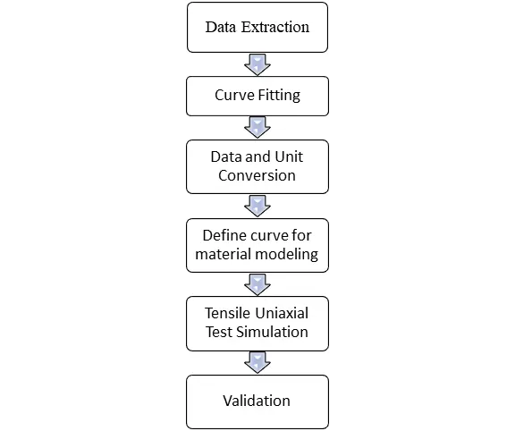
Figure 1: Methodology followed in the work for the material modeling.

PROCEDURE

The material test data are always collected in the form of force-displacement or stress-strain. If the data has all the data points in it, it is always good, but if the data is available in some other format, then it has to be extracted. In this work, the stress-strain plot of the graphite iron casting material was available in the image form, as shown in the figure below.

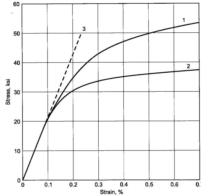
Figure 2: Stress-Strain plot of the graphite iron casting material at different strain rates.

Now as the data was available in image format, it was extracted using GetData Graph Digitizer, and the plots of curve 1 were brought to an excel file, as shown in the figure below. In fig. 3, the engineering stress-strain curve is curve 1 from fig. 2. But to introduce the curve in LS-Dyna, it has to be de-noised or it should be monotonically increasing. The engineering stress-strain curve in fig. 3, however, has some noise in it, and thus couldn’t be provided as input. Therefore, curve-fitting was required.

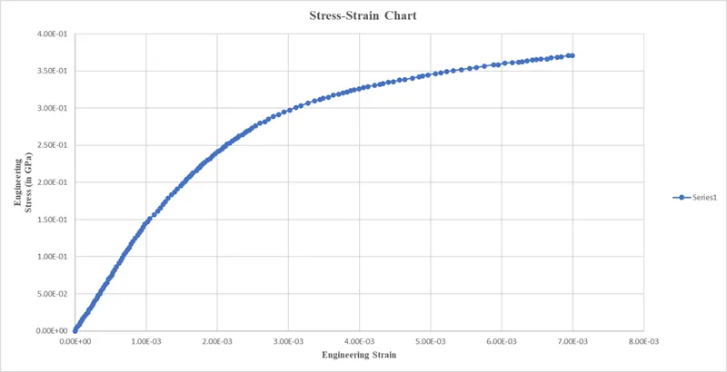
Figure 3: Engineering Stress-Strain curve.

Further, when the distinct point of linear to non-linear cannot be found out, to know the value of yield stress, 0.2% offset linear curve, parallel to the elastic region of the engineering stress-strain curve is drawn. But in this case, the effective stress (ES) vs. effective plastic strain (EPS) plot was drawn to find out that till how much stress, there is no significant change in strain. Below shown equations were used to derive the values of EPS and ES.

True Stress = Engg. Stress * (1 + Engg. Strain)

True Strain = ln (1 + Engg. Strain)

Effective Stress (ES) = True Stress

Effective Plastic Strain (EPS) = True Strain – (True Stress/ E)

After deriving the required value of ES and EPS, the curve of ES vs. EPS was plotted, as shown below.

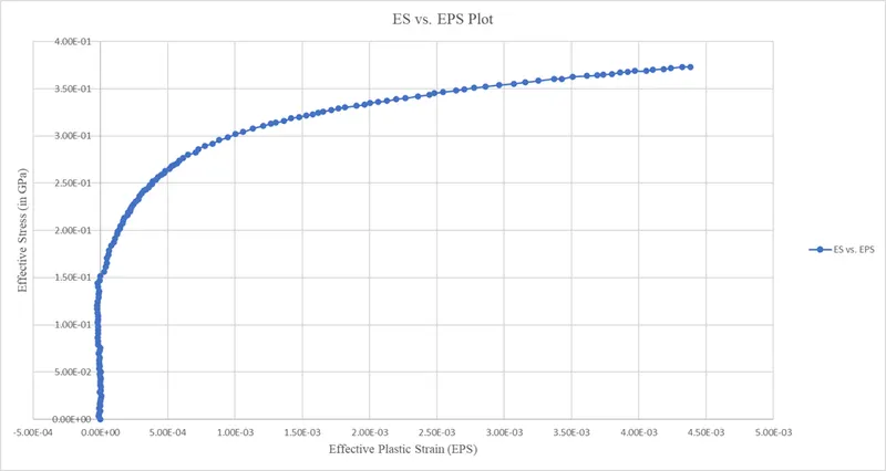
Figure 4: Effective Stress vs. Effective Plastic Strain plot.

From figure 4, it can be observed that till 0.15 GPa of effective stress value there was no significant change in strain. The non-linear curve started after 0.15 GPa of stress value, thus it was considered as an input data points for ls-dyna. Figure below shows the plot that was taken as an input to ls-dyna.

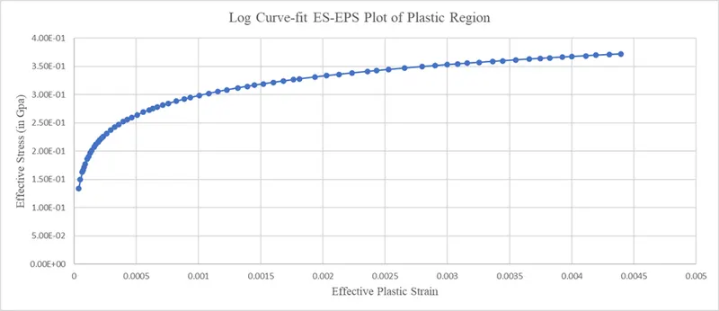
Figure 5: The input plot for material modeling in ls-dyna.

A tensile test was performed on dog bone specimen using the data collected from the experiment, to find out the accuracy of the material modeling. To do that, the dog bone specimen was imported into ls-dyna. As a part of the preprocessor, a 024-PIECEWISE LINEAR PLASTIC material card was selected to assign the material data collected from the experiment, to the specimen. The card is shown in the figure below. After this, the SECTION card was created to assign it a thickness of 1 mm.

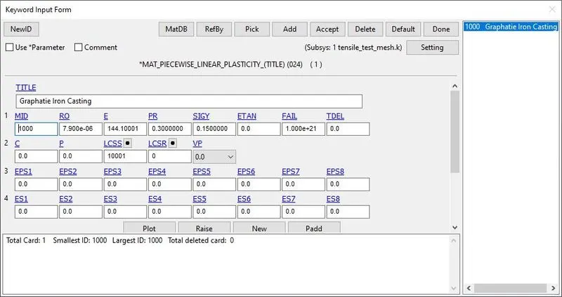
Figure 6: 024-Material card with the LCSS defined.

In boundary condition, to perform the uniaxial test similar to the test that is performed on the UTM testing machine, one end of it is fixed and the other end is given the displacement of 1 mm.

As a part of controlling the solver, *CONTROL_TERMINATION card was provided with the end time of simulation equal to 1s. The simulation had to run implicitly, thus the *INCLUDE_IMPLICIT_GENERAL card was introduced. For the output in, *DATABASE_BINARY_D3PLOT card was called, and along with that in *DATABASE_ASCII_option card, GLSTAT, MATSUM, and ELOUT was called.

Post-processing

The figure below shows the von-mises contour of the uniaxial tension in the dog bone specimen, with the maximum stress of 0.37 GPa.

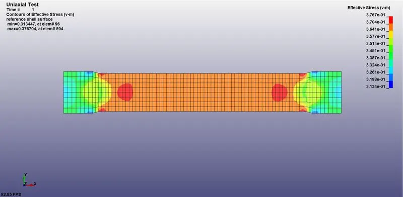
Figure 7: Von-Mises contour of the uniaxial test on the dog bone specimen.

The second objective of this work was to get the eff stress vs. effective plastic strain plot of the simulation and compare it with the experimental result. The effective stress and the effective plastic strain plot of the element, present at the middle of the specimen, is shown below.

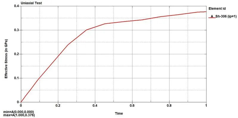
Figure 8: Effective stress vs. time plot.

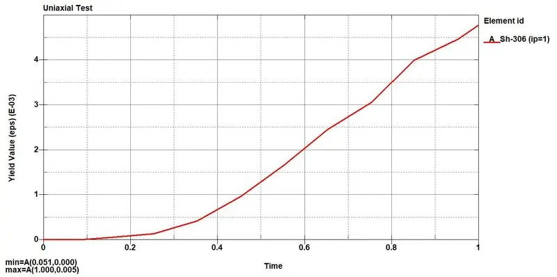
Figure 9: Effective plastic strain vs. time plot.

When both the effective stress and the effective plastic strain plots are available, they can now be brought into one plot.

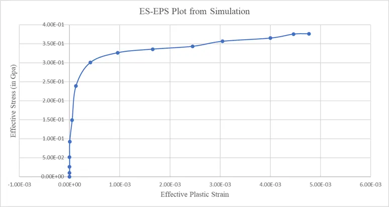
Figure 10: Effective stress vs. effective plastic strain plot obtained from the simulation.

After obtaining the plot of effective stress vs. effective plastic strain from the simulation, it has to be compared with the experimental plot of ES-EPS, to study how much it is deviating from the experimental results. The figure below shows the plot of effective stress and effective plastic strain obtained from simulation and the experiment.

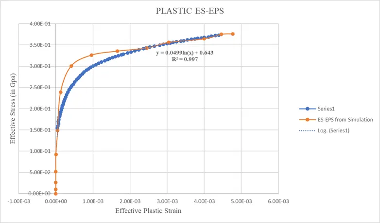
Figure 11: Comparison of ES-EPS plot obtained from experiment and simulation.

CONCLUSION

From experimental results, the stress (in ksi) vs. strain (in %) plot was available. It had to be modeled in the software. To use it as a plastic material model, the yield value has to be known. Also, the ls-dyna only takes effective stress and the effective plastic strain value, and not the engineering stress and the engineering plastic strain value. Thus, using the bunch of formulas, the engineering stress-strain value was converted to an effective stress-strain value. These values showed the elastic and plastic regions. Thus the plastic region was separated. LS-Dyna also doesn't take noisy data. The data has to be monotonically increasing. Thus, using logarithmic curve-fit, the denoised curve was used as an input to ls-dyna.

The uniaxial tensile test was again run virtually, and the values of effective stress and effective plastic strain values were drawn out. It was then compared with the effective stress and effective plastic strain values of the experimental result, as can be seen in fig. 11. The results from the virtual test have shown a significant deviation from the experimental result, up to a certain point, after which it is perfectly matching with the experimental result. This shows that the material that was modeled can be used for further analysis, but with slight modification.