Week - 9 Material Modeling from Raw Data

                                                 week-9 (Material modeling from Raw data)

AIM

 To do material modeling for the given true stress-strain curve of graphite iron casting, by using the given material card MAT-24 and then validate the simulated material model data with the experimental material model raw data.

MATERIAL MODELLING

Material modeling is a widely used, technique in industries particularly in the areas of Research and development.  It involves testing a new material by experiments to estimate its behavior in terms of the stress-strain curve and process the experimental raw data and input the processed data to software like LS-DYNA to see its behavior. Finally, the simulated behavior of the newly modeled material is validated with the experimental test data.

ADVANTAGES OF MATERIAL MATERIAL MODELLING 

• Experiments repeatability for testing the materials can be avoided.
• with material modeling, there is an improved life cycle, fatigue, thermal, wear-resistant and it can eliminate manufacturing cost.
• The newly developed material models can be used for (buckling, linear, static & thermal analysis.

PROCEDURE 

Extraction of Raw Data

•  Initially, the stress-strain curve of graphite iron casting is opened as an image.

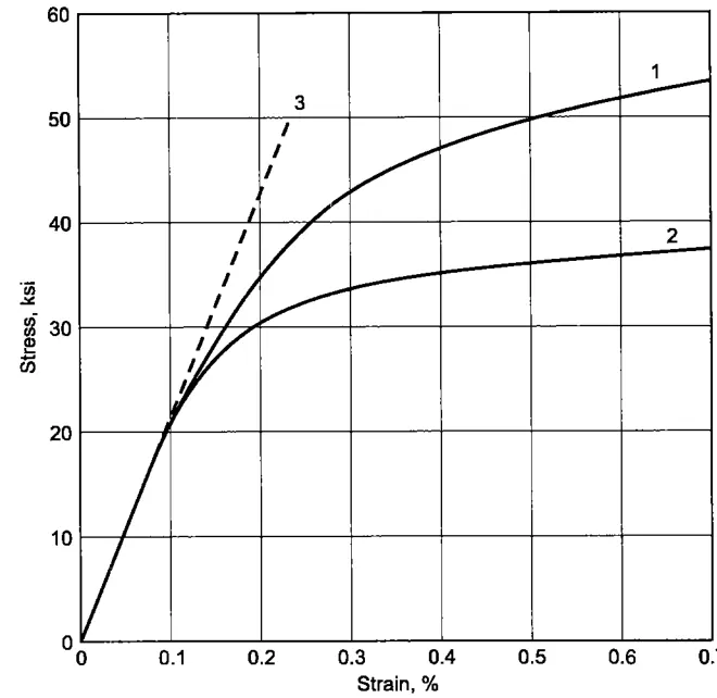
                      Fig, represents the stress-strain curve of graphite iron casting.

• Now, the raw test data has to be collected or it should be extracted from the image by using the get data graph digitizer app.
• Here, we choose curve 1, to extract the data from the image. 

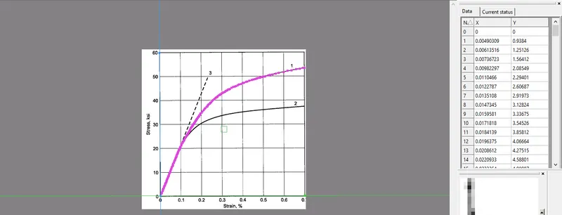
      Fig, represents the data extracted for curve 1, from the get data graph digitizer app.

• Now, the extracted data is exported to the MS-EXCEL, the extracted data contains stress and strain values. Here we extracted about 188 data values containing stress and strain values.
• In the given extracted data, the stress and strain are expressed in Ksi and in % and the data has to be converted into the given unit system which is kg-mm-ms.

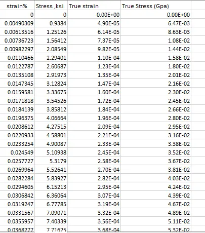
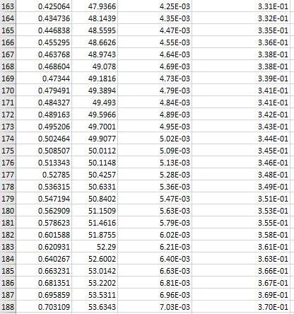
Figures represent the raw data and converted test data 

• The stress data has been converted to our unit system and the stress values are expressed in Gpa.

DATA CLEANUP

• The extracted test data could be noisy, if we plot a curve, the curve will not be smooth, and in order to avoid we need to filter the unwanted data to bring a smooth curve.
• The process of filtering the data and cleaning up is called curve fitting.
• Here, the curve fitting is done in excel to ensure that the extracted data is smooth or not.
• Here, the curve fitting is done by using a polynomial function with a higher-order 3 to fit the curve with better accuracy.

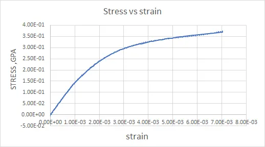
Fig, represents the curve fitting of the extracted data with a higher-order (3)

polynomial function.

• Here, the stress values are converted to Gpa.
• Now, the stress-strain, data is ready for inputting in LS-DYNA.

DEFINING NEW MATERIAL DATA IN LS-DYNA & CONDUCTING A TENSILE TEST TO DOG BONE SPECIMEN FOR VALIDATING

• The given dog bone specimen is opened in the LS-PREPOST.

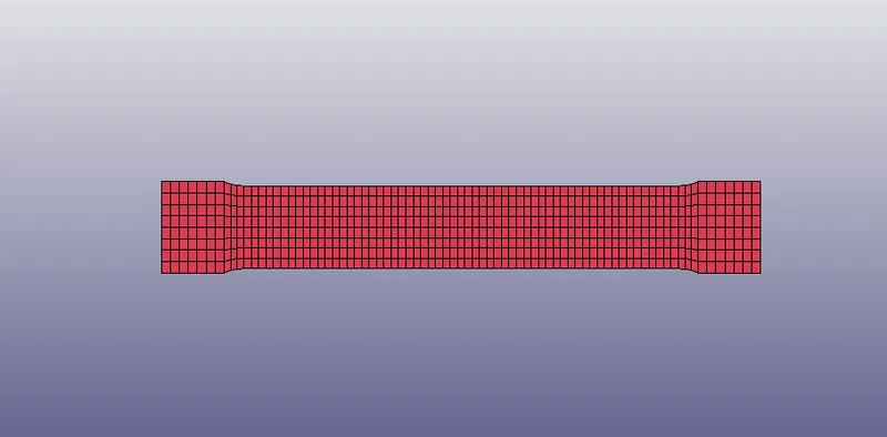
Fig, represents the dog bone specimen in LS -DYNA 

• Now, we need to input, the extracted Material data in the LS-DYNA in the MAT-24 material card.
• Before, inputting the data we need to define the parameters such as density, Elastic modulus, yield stress, Tangent modulus, LCSR, and other parameters for referencing the material.

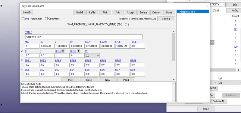
Fig, represents the material parameters that are defined in MAT-24 card 

• The material parameters are been converted to the unit system (kg-mm-ms) and the material properties of steel are assigned.

                                  RO = 7.83e^-6

                                  E =  144 Gpa

                                PR= 0.33

                   Yeild stress = 0.15 Gpa

•  After inputting the material properties , the extracted test data are defined or loaded in the define curve.
• For this defining operation, the model is edited in the notepad++ and the extracted data is loaded in the notepad++.   

       

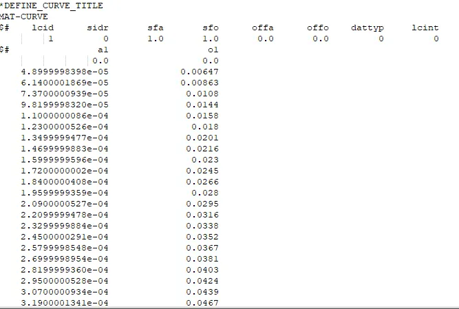
Fig, represents the defining of extracted data into the define curve.

• After defining the curve, the curve is loaded and plotted to check whether the curve is well defined or not.

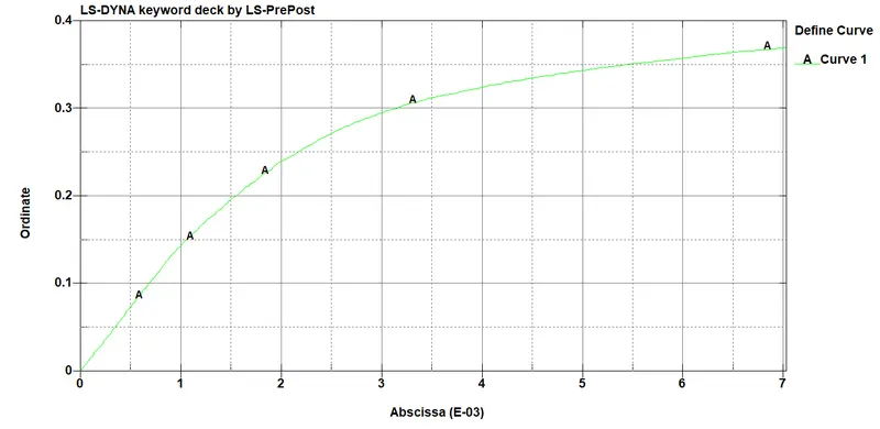
Fig, represents the loaded curve of the extracted data.

• once, everything is done, now apply boundary conditions to the dog bone specimen.
• Now, for conducting the tensile test, the dog bone specimens is fixed at the one end and its y (lateral) nodes constrained are allowed to freely at the top and at the bottom and while the middle nodes are fixed.

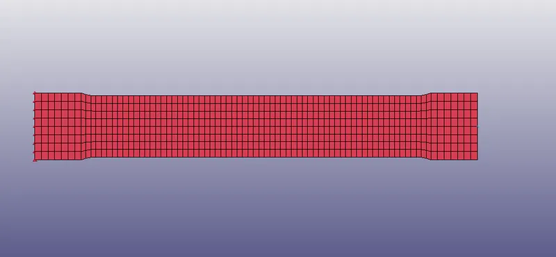
Figure, represents the nodes that are constrained in the (Y) one end and at the middle at the both the ends .

• The nodes are allowed to move freely, in the lateral direction when the displacement is applied.

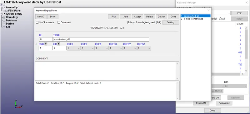
Fig,represents the nodes that are allowed to move freely in the Y-direction.

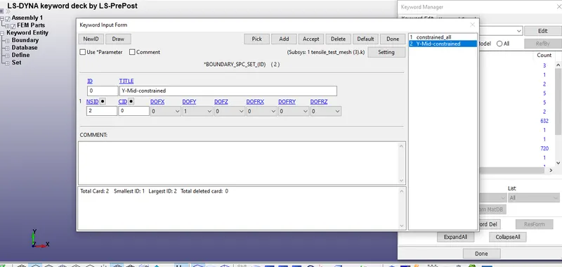
Fig, represents the Middle Y constrain of the nodes at the both the ends.

• In the section , the section shell is selected with the element formulation 2 .

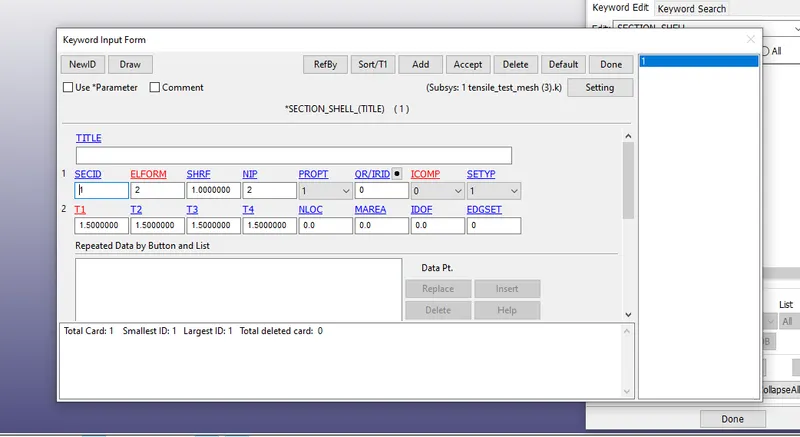
Fig, represents the section shell is defined.

• After , assigning the section , go the part and assign the material and sec ID to the part.
• Before , giving the initial displacement now we need to calculate the stretch .

                                 e= dl / l

                               0.7 /100 = dl/145

                                  e= 0.7/100

                                 e= 0.007 

                     Length of the specimen =145 mm

                              dl = 1.015 

• Now , we need to define the displacement in the define curve option.

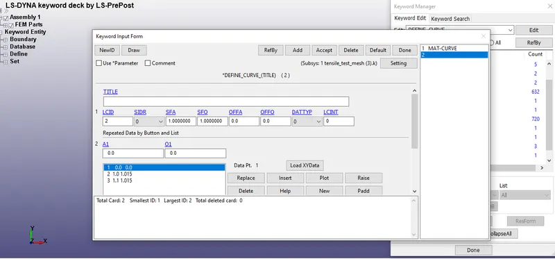
Fig, represents the defining the displacement in the define curve option.

• Then , check whether the curve is plotted correctly or not.

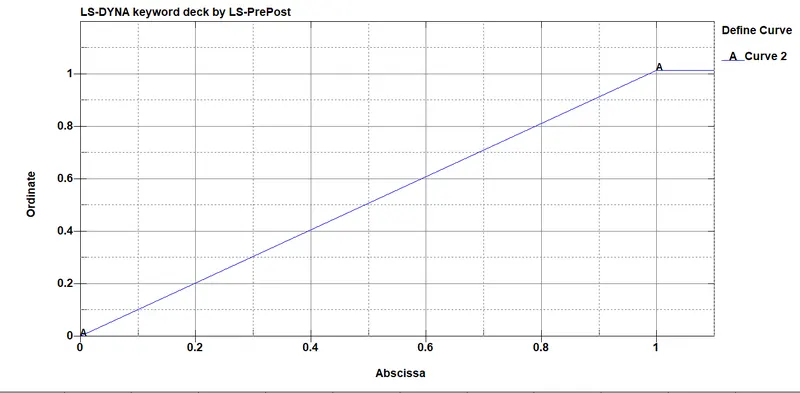
Fig , represents the displacemement defined in the define curve option.

• once ,everything is done now we need to define the terimination time in the problem .

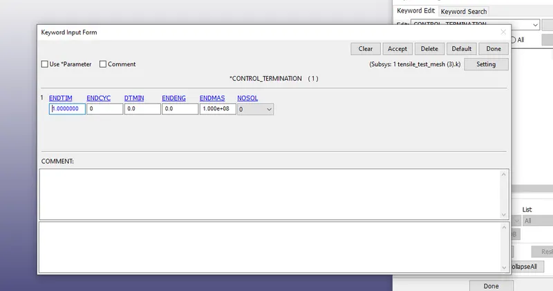
Fig, represents the terimination time defined in the control terimination card.

• once ,everything is done we need to activate the impicit analysis for solving the problem.
• For that , we need activate the implicit auto card for optimizing the number of iterations for solving the problem in a small interval.

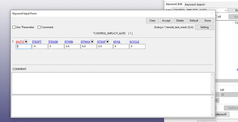
Fig , represents the ITEOPT and ITEWIN defined in the control implicit card.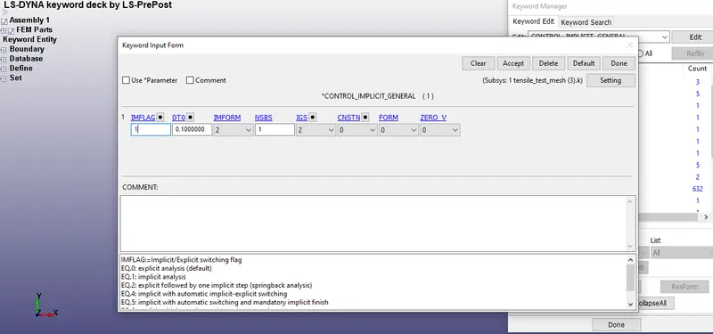

Fig, represents the activation of IMFLAG and assignment of dt in the control implicit general.

• Then, activate other implicit cards such as implicit general and implicit solver for solving the non-linear problem.

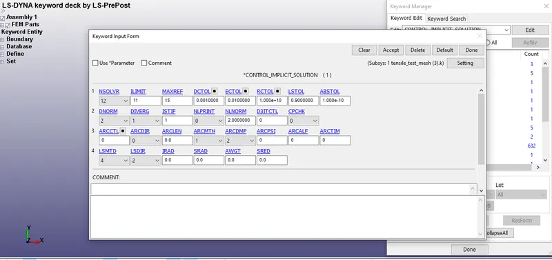
Fig, represents the activation of the control implicit solution card.

• Here, we activate the Nsolver (12) for activating the non-linear analysis.

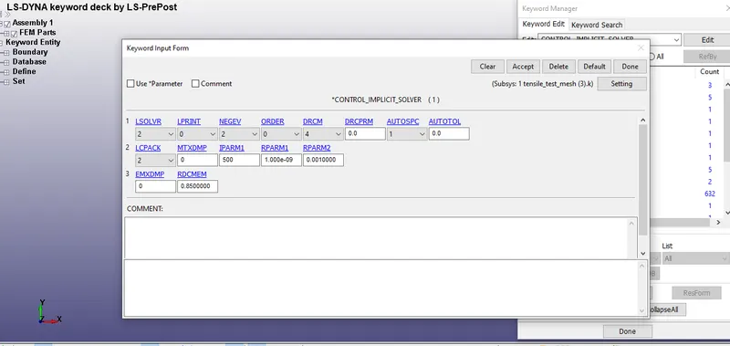
Fig, represents the activation of control implicit solver.

• Here, we activate the control implicit solver to solve or run the non-linear problem.
• Finally, we need to define the required output in the ASCII option.

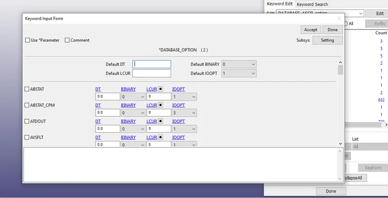
 Fig, represents the assignment of GLSTAT and ELOUT in the ASCII option.

• The outputs are defined with the interval of 0.01 
• Then, the output is defined with the binary d3 plot option.

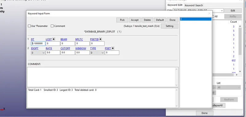
 Fig, represents the defining of database binary D3 plot.

• Here, we define the output with the dt interval of 0.1 for getting the output.
• Finally, the problem is solved using LS - Run and we got the normal termination of the model.

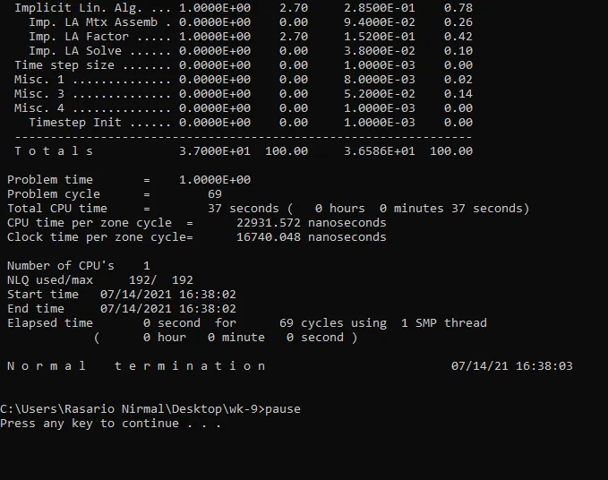
Fig, shows the normal termination of the model.

RESULTS 

 ANIMATION OF THE DOG SPECIMEN 

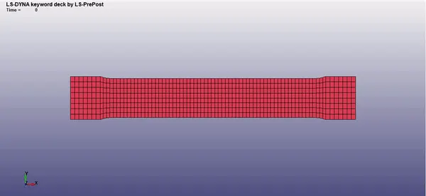
fig represents the animation of dog bone specimen with displacement

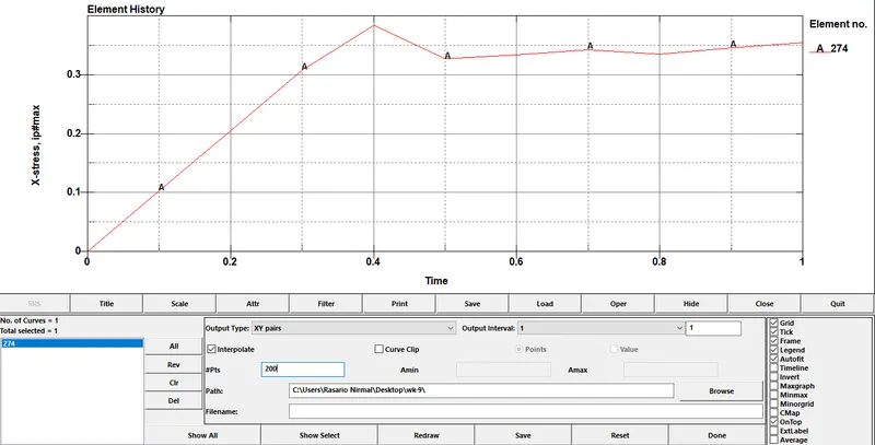
                               Fig, represents the x- stress vs time 

• The x-stress is the curve is obtained from the displacement which we have given as an input.
• From, the x-stress curve we interpolate around to 200 points to plot the stress-strain curve in the MS -excel sheet for validating against the test data.
• The x-stress values which we obtained are saved in the notepad++ and the values of x-stress are exported to the MS-EXCEL Sheet to plot the stress-strain curve.

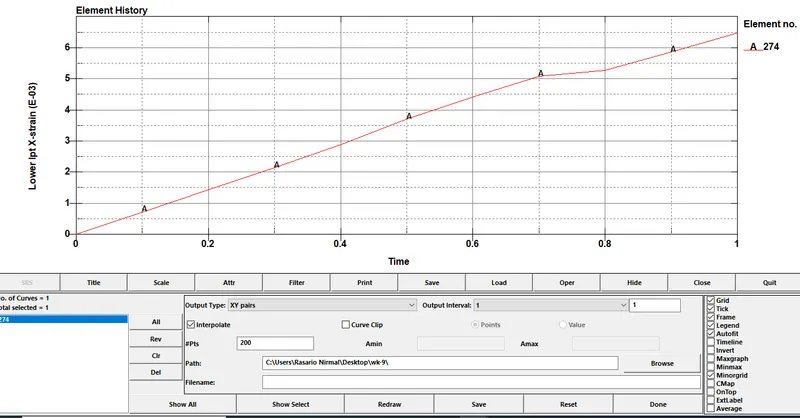
                                    Fig, represents the lower_ipt_strain vs time 

• In a similar fashion, the strain values are extracted and exported to the MS-EXCEL Sheet.

         

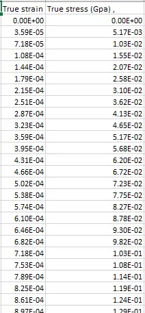
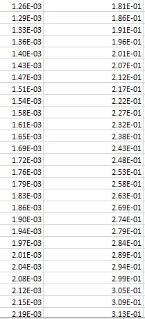
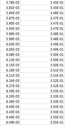
• Fig, represents the stress and strain values that are obtained from the simulation.
• From, the figure it is understood the stress and strain values are obtained by giving an initial displacement for the dog bone specimen.
• once, the values are exported to the excel sheet, now we need to plot the stress-strain curve for the newly developed material model, in the excel sheet.

 

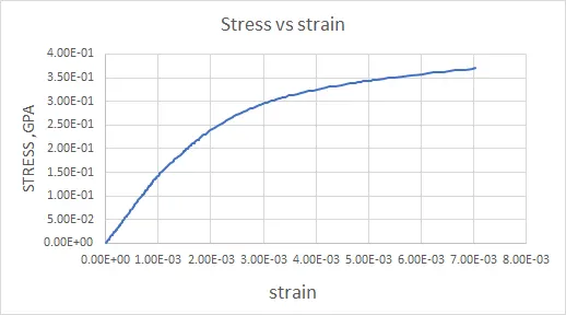
 Fig, represents the stress-curve of the extracted data from the experimental testing

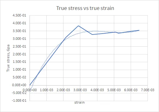
Fig, represents the stress-strain curve of the newly modeled material using MAT24

• From, the figures it is evident that the maximum stress occurs around 0.38 Gpa for the newly modeled material with the strain of 0.00029 and whereas for the extracted data the maximum stress was found to be around 0.37 Gpa and with the strain of 0.0007
• As we, see that the stress-strain curve of the newly modeled matches only with some stress-strain values of the experimental test data and we can see a large variation between the experimental stress-strain curve and with the newly modeled material stress-strain curve.
• The reason why we find such differences or variations in the curve is,  experimental testing is done with the actual material properties and whereas, in the simulation, the material properties (such as E, density & other parameters) differ, when compared to the material properties of actual testing. Hence, we find a smooth curve on the extracted experimental data and whereas, we cannot find a smooth non-linear curve for the newly modeled material.
• In order to match, the curve we need to have proper material parameters and material constants to bring a smooth curve in the newly modeled material.

CONCLUSION

• Thus, the material is modeled by using a MAT-24 card, the stress-strain of the newly modeled material is validated against the stress-strain curve of the graphite iron casting which is obtained through experimental testing. The required outputs are obtained and then the stress curves are compared against each other and then recommendations are suggested to obtain a smooth curve for the newly modeled material.