Week - 9 Material Modeling from Raw Data

AIM:

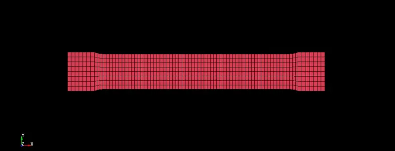
To create a material model using the data extracted from the given true stress-strain curve of graphite iron casting and validate it using the dog bone specimen.
Note: The unit system used is kg-mm-ms.

INTRODUCTION:

• To get realistic results for any analysis using FEA, a good material model for the material is necessary. A material model can have all sorts of data describing the behavior of the material in different conditions: say different tensile test curves for different strain rates and much more. This helps getting realistic behavior of the component with the material model in all sorts of situations.
• Building a material model requires test data from various experiments conducted in real life to describe the material behavior in detail. A complex analysis would benefit from a detailed material model, whereas a simpler simulation would not benefit much. The data collected from an experimental test is first cleaned to make sure any unnecessary data points are filtered out to get clear picture. Usually, the same test is repeated a number of times to ensure repeatability of the results. This test data is then inserted in the suitable format into a model: say effective stress-strain curve in x-y co-ordinates.
• A cleaner data with consistence behavior in the case of a stress strain plot, inconsistent data points should be avoided as it can affect the stability if the simulation having such a material model. A fitted curve with 98%+ accuracy can solve such issues. After matching for the unit system of the analysis, this data can be added to the simple material model to make it more detailed – for example with the use of material model such as MAT24 – linear piecewise material.
• A good practice of the material modelling procedure is the validation of the model. By performing simple analysis for which an experimental test can be performed or such data can be acquired, and then comparing the experimental and analysis results gives a good benchmark for the model. In this exercise, we try and replicate such a process.
• Material modeling is done with the help of raw data. We have to extract the data from given image. The given image gives you the Engineering Stress and Engineering Strain values. These values will produce the True stress and true strain with the help of calculations.

Given model-

Dogbone-Specimen

PROCEDURE :

Steps -

1. Extract the data from the diagram.
2. Clean the data and visually confirm that it matches the original data.
3. Convert the data to (kg-mm-ms) unit system
4. Process the data and create the material as demonstrated
5. Use the material model with a dog-bone specimen and validate the same.

1. Data Extraction:

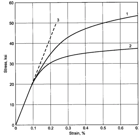
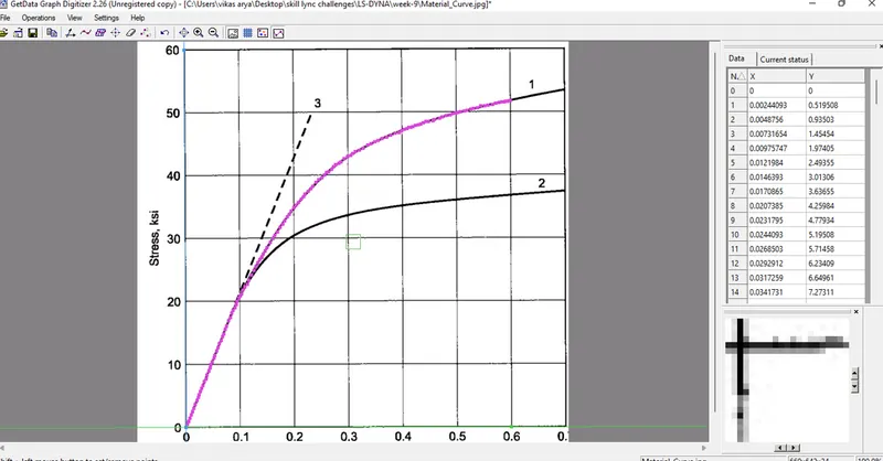
The given image file of true stress-strain graph of graphite iron casting is opened in data digitizer software to extract the data and export it as excel file.

The curve 1 is chosen to extract data of stress-strain of graphite iron casting as shown in fig.1.

Note: Ensure the data points picked is evenly spaced so as to get smooth curve and better convergence.

Extracted Raw Data Values-

Strain%	Stress (ksi)
0.00366	0.83
0.0109	2.07
0.0146	2.9
0.0195	4.15
0.0256	5.39
0.0292	6.22
0.0341	7.16
0.0402	8.51
0.0439	9.44
0.0475	10.2
0.0524	10.9
0.056	11.9
0.0621	13.2
0.0682	14.3
0.0706	14.9
0.0743	15.7
0.078	16.6
0.0828	17.4
0.0865	18.5
0.0913	19.1
0.0938	19.7
0.0962	20.2
0.0999	20.8
0.103	21.5
0.107	22
0.112	22.8
0.118	23.8
0.124	24.7
0.131	25.8
0.14	27.1
0.147	28.1
0.154	29
0.162	30
0.168	30.9
0.175	31.6
0.181	32.5
0.188	33.4
0.193	34
0.2	34.6
0.208	35.5
0.215	36.3
0.222	37
0.233	38.1
0.24	38.7
0.248	39.3
0.256	39.9
0.262	40.4
0.272	41.2
0.284	41.9
0.292	42.5
0.3	42.9
0.308	43.4
0.318	43.9
0.329	44.4
0.342	45
0.354	45.4
0.366	45.8
0.377	46.3
0.385	46.6
0.395	47
0.401	47.2
0.407	47.4
0.415	47.5
0.423	47.8
0.435	48.2
0.445	48.4
0.456	48.7
0.466	49
0.476	49.2
0.486	49.5
0.5	49.8
0.512	50
0.531	50.6
0.541	50.8
0.554	51.1
0.565	51.3
0.575	51.5
0.586	51.7
0.601	51.9
0.612	52.1
0.625	52.3
0.634	52.5

Stress VS Strain% graph-

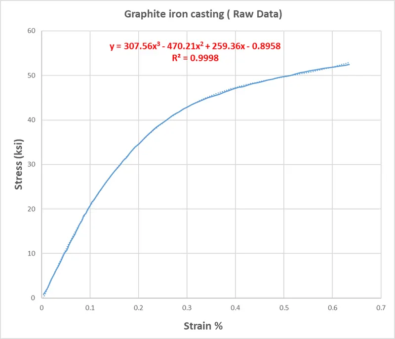
Fig-1

By using the raw data values a graph has been obtained with the help of an Excel sheet as shown in Fig-1. But the obtained graph is not smooth because the extracted raw data is not proper or it is noisy data. So, we can use the curve fit option using an Excel sheet and obtain the equation for the fit curve and extract nice smooth data.

Strain%	Stress (ksi) y = 307.56x3 - 470.21x2 + 259.36x - 0.8958
0.00366	0.047173934
0.0109	1.875756649
0.0146	2.791583205
0.0195	3.985203166
0.0256	5.440819175
0.0292	6.284249494
0.0341	7.413806424
0.0402	8.790574408
0.0439	9.609931552
0.0475	10.39585047
0.0524	11.44783125
0.056	12.2077939
0.0621	13.47078886
0.0682	14.70305495
0.0706	15.17954916
0.0743	15.90501102
0.078	16.61947557
0.0828	17.53011408
0.0865	18.21966856
0.0913	19.09831128
0.0938	19.54888085
0.0962	19.9769154
0.0999	20.62820174
0.103	21.16590123
0.107	21.84905994
0.112	22.68630542
0.118	23.66680688
0.124	24.62129232
0.131	25.70250906
0.14	27.04242864
0.147	28.04632352
0.154	29.01742996
0.162	30.08792871
0.168	30.8638093
0.175	31.74034813
0.181	32.46756133
0.188	33.28841308
0.193	33.85689408
0.2	34.62828
0.208	35.47561993
0.215	36.18778937
0.222	36.87331908
0.233	37.8982794
0.24	38.51821344
0.248	39.19689438
0.256	39.84467799
0.262	40.3108077
0.272	41.05133254
0.284	41.8822451
0.292	42.40268295
0.3	42.89742
0.308	43.36740109
0.318	43.92150375
0.329	44.49024743
0.342	45.11059672
0.354	45.63673853
0.366	46.12152893
0.377	46.53231752
0.385	46.81233394
0.395	47.14176911
0.401	47.32915997
0.407	47.50933533
0.415	47.73903397
0.423	47.95755848
0.435	48.26646059
0.445	48.50859796
0.456	48.76124849
0.466	48.98047794
0.476	49.19165917
0.486	49.39663754
0.5	49.6767
0.512	49.91379418
0.531	50.29175845
0.541	50.49560687
0.554	50.76954471
0.565	51.01198792
0.575	51.24305813
0.586	51.51124286
0.601	51.90491651
0.612	52.21737438
0.625	52.61630938
0.634	52.91333163

Graph Obtained-

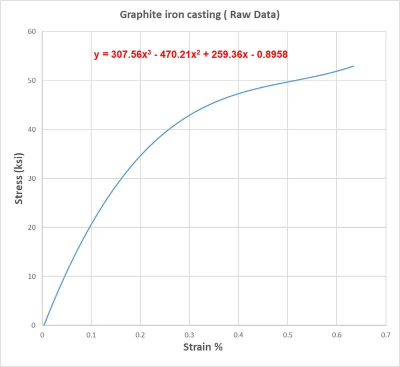
Fig-2

Now we can see that the graph obtained is very much smooth and we can proceed further and convert the units of the data as per requirement.

CONVERTING UNITS (kg-mm-ms)-

converting the stress unit given values for stress are in terms of (ksi) and we have to convert it to (GPA).

1Ksi= 0.0068947573Gpa

Also calculating strain from the strain %, by dividing the strain % values by 100 as shown in the table below.

Strain	Stress (GPA)
0.0000366	0.000325253
0.000109	0.012932887
0.000146	0.019247289
0.000195	0.027477009
0.000256	0.037513128
0.000292	0.043328375
0.000341	0.051116396
0.000402	0.060608877
0.000439	0.066258146
0.000475	0.071676866
0.000524	0.078930018
0.00056	0.084169776
0.000621	0.09287782
0.000682	0.101373995
0.000706	0.104659307
0.000743	0.109661191
0.00078	0.114587251
0.000828	0.120865882
0.000865	0.125620193
0.000913	0.131678221
0.000938	0.134784789
0.000962	0.137735983
0.000999	0.142226445
0.00103	0.145933752
0.00107	0.150643965
0.00112	0.15641657
0.00118	0.16317689
0.00124	0.169757835
0.00131	0.177212562
0.0014	0.186450982
0.00147	0.193372594
0.00154	0.200068137
0.00162	0.207448966
0.00168	0.212798474
0.00175	0.218841997
0.00181	0.223855956
0.00188	0.229515529
0.00193	0.233435068
0.002	0.238753586
0.00208	0.24459579
0.00215	0.249506025
0.00222	0.254232586
0.00233	0.261299439
0.0024	0.265573733
0.00248	0.270253074
0.00256	0.274719384
0.00262	0.277933236
0.00272	0.283038975
0.00284	0.288767915
0.00292	0.292356208
0.003	0.2957673
0.00308	0.299007705
0.00318	0.302828109
0.00329	0.306749458
0.00342	0.311026616
0.00354	0.314654236
0.00366	0.317996748
0.00377	0.320829036
0.00385	0.322759681
0.00395	0.325031057
0.00401	0.326323071
0.00407	0.327565337
0.00415	0.329149053
0.00423	0.330655726
0.00435	0.332785531
0.00445	0.33445501
0.00456	0.336196974
0.00466	0.337708508
0.00476	0.339164551
0.00486	0.340577827
0.005	0.34250879
0.00512	0.344143497
0.00531	0.346749469
0.00541	0.348154954
0.00554	0.350043689
0.00565	0.351715276
0.00575	0.353308449
0.00586	0.355157518
0.00601	0.357871802
0.00612	0.360026123
0.00625	0.362776683
0.00634	0.364824579

we calculate the young modulus by slope of the linear elastic region

young modulus = 141.227 GPA

we need to define the yield limit from the graph it is observed that the material linear elastic region end at about 20 ksi so our yield limit is 0.142226445 GPA , from this point we define the plastic region. In LS DYNA plastic region is defined by curve between EFFECTIVE PLASTIC STRAIN vs TRUE STRESS(corresponding to the strain).

Calculation of EFFECTIVE PLASTIC STRAIN and TRUE STRESS-

True strain = ln(1+ engineering strain)

Effective plastic strain = total true strain - ((true stress) / (young modulus))

True stress = (engineering stress)*(1+ engineering strain)

Effective Strain	Stress (GPA)
1.61E-06	0.150805155
1.06E-05	0.156591756
2.25E-05	0.163369438
3.57E-05	0.169968335
5.27E-05	0.17744471
7.70E-05	0.186712014
9.77E-05	0.193656852
0.000119992	0.200376242
0.000147405	0.207785033
0.000169276	0.213155976
0.000196183	0.21922497
0.000220416	0.224261135
0.000250026	0.229947018
0.000272043	0.233885597
0.000304055	0.239231093
0.000342304	0.245104549
0.000377192	0.250042463
0.000413373	0.254796982
0.00047277	0.261908266
0.000512137	0.26621111
0.000558576	0.270923301
0.000606516	0.275422666
0.000643428	0.278661421
0.000706714	0.283808841
0.00078546	0.289588016
0.000839585	0.293209888
0.000894957	0.296654602
0.000951532	0.299928649
0.001023871	0.303791102
0.001105423	0.307758664
0.001204316	0.312090327
0.001297858	0.315768112
0.001393406	0.319160616
0.001482621	0.322038561
0.001548413	0.324002306
0.001631649	0.326314929
0.001682088	0.327631627
0.001732876	0.328898528
0.001801102	0.330515021
0.001869868	0.3320544
0.001973928	0.334233149
0.002061381	0.335943335
0.002158236	0.337730032
0.002246787	0.339282229
0.00233572	0.340778974
0.002424945	0.342233035
0.002550179	0.344221334
0.00265765	0.345905512
0.002827651	0.348590708
0.002916866	0.350038472
0.00303239	0.351982931
0.003129603	0.353702467
0.003217441	0.355339973
0.003313361	0.357238741
0.003442764	0.360022612
0.003536475	0.362229483
0.003645746	0.365044037
0.003720359	0.367137567

Obtained graph-

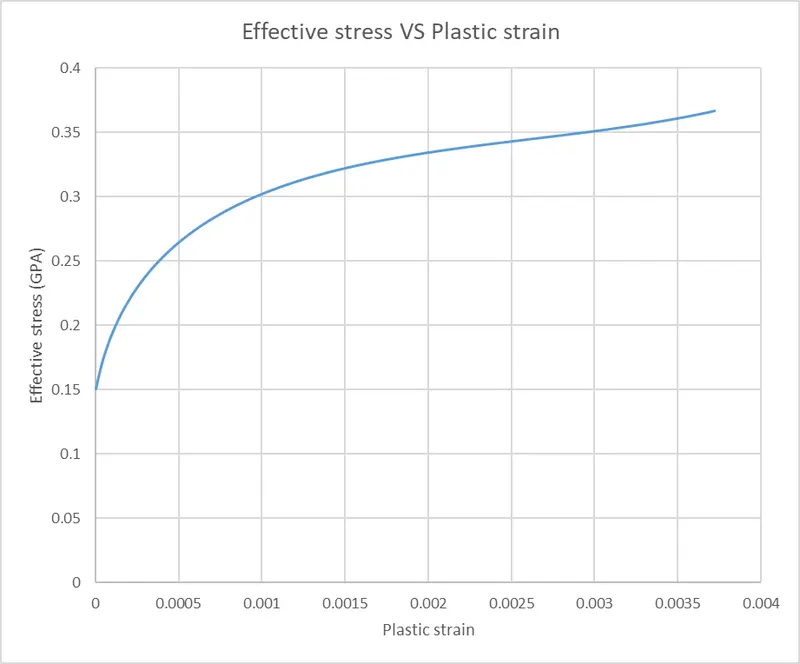
Fig-3

Model setup-

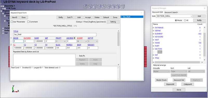
Section:

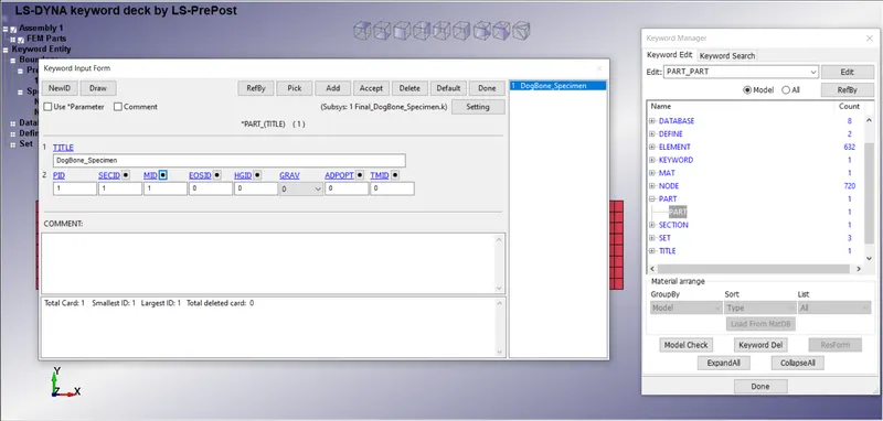
Create a shell section for the specimen.Assign section id and material id to the part.

Define:

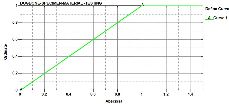
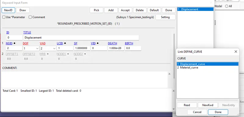
The keyword DEFINE provides a way of defining boxes, coordinate systems, load curves, functions, tables, transformations, and orientation vectors. The curve option was selected, and the assigned value of load-displacement is presented in the following card.

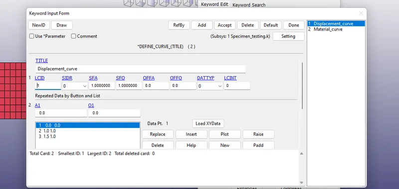
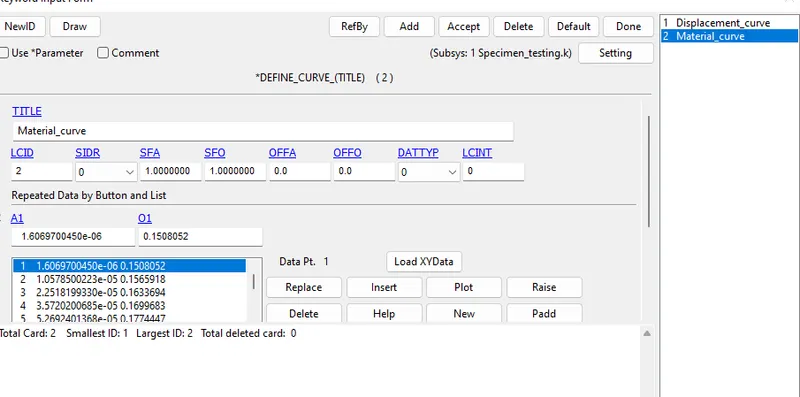
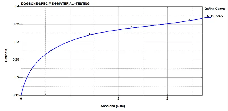
Now we have to define the material load curve which we have formulated from the Raw data-

Material:

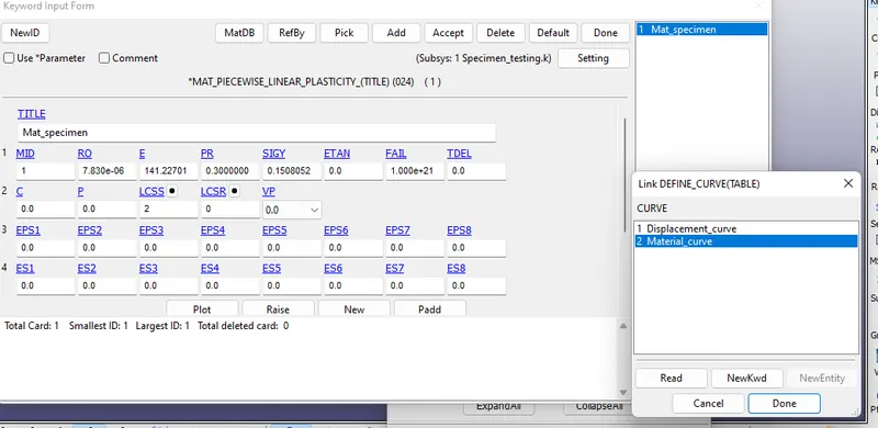
Here we will use a MAT24 card to create the material card.

Input the values of density, poisons ratio, and yield strength below. Also for defining the plastic region we will use the material curve defined above instead of the tangent modulus.

Assigning Section and Material:

Section and Material are assigned to the part.

8.Boundary:

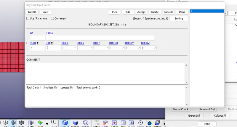
The keyword BOUNDARY provides a way of defining imposed motions on boundary nodes. The Prescribed Motion Set Displacement boundary condition was defined for the challenge purposes and respective curve is assigned to the card. A node set is created out of the edge and allowed to move in X-direction.

9.Control Cards:

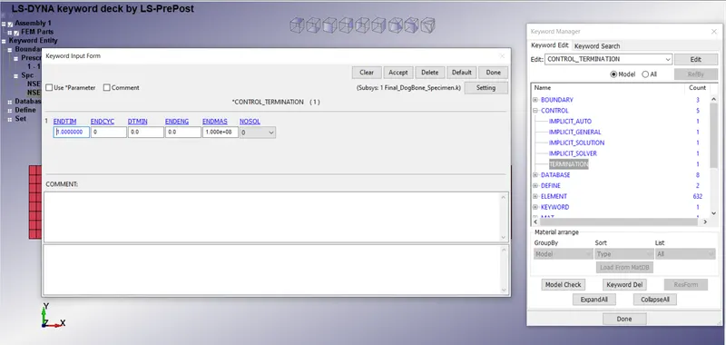
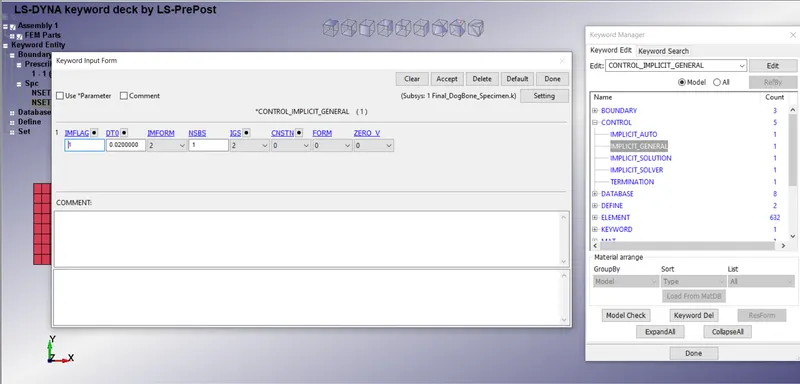
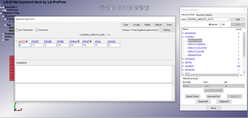
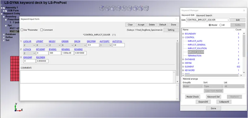
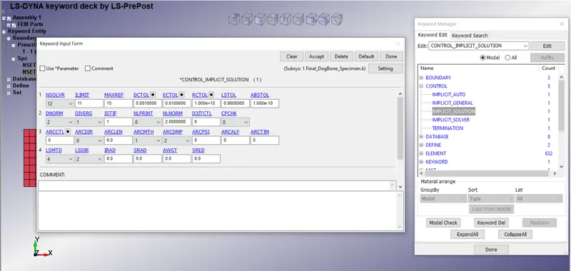
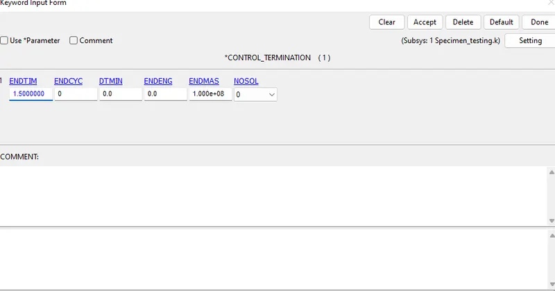
The keyword control cards can be used to change defaults. The Implicit Auto, Implicit General, Implicit Solution, Implicit Solver, and Control Termination cards were created for the challenge purposes.

Database Cards:

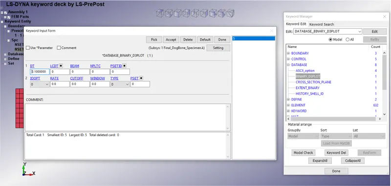
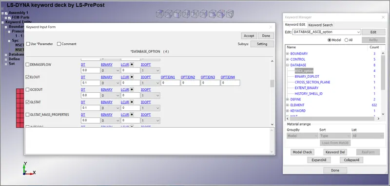
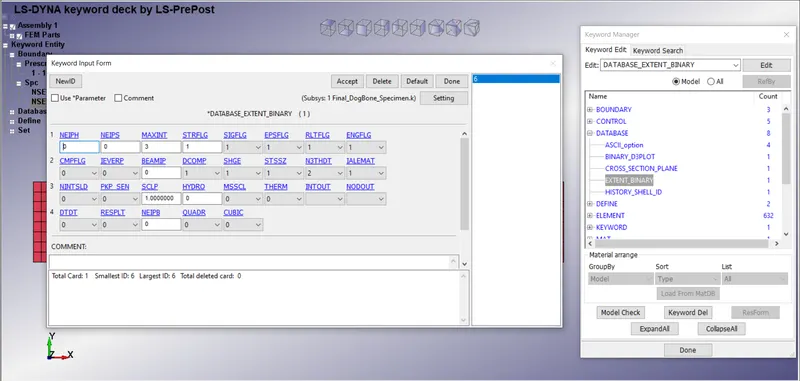
The database definitions are necessary to obtain output files containing results information. The binary D3Plot, Extent Binary, and ASCII options were selected for the challenge purposes.

Providing termination time-

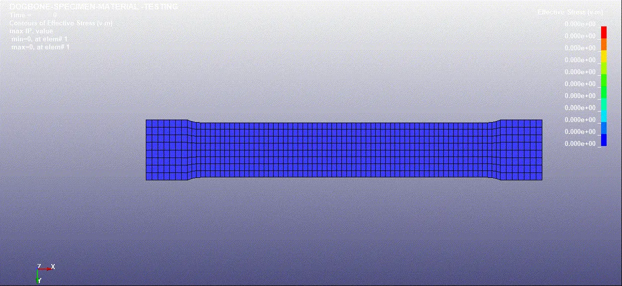
SIMULATED RESULTS-

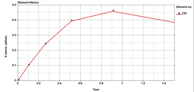
Stress vs. Time Plot:

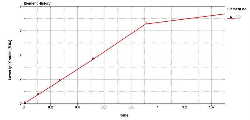
Strain vs. Time Plot:

EFFECTIVE PLASTIC STRAIN VS EFFECTIVE STRESS FROM THE SIMULATED RESULTS-

Effective Strain	Stress (GPA)
0	0
6.56483E-08	0.026190627
1.31297E-07	0.052381255
1.96957E-07	0.078571878
4.80212E-06	0.104137905
2.75653E-05	0.127205521
5.03286E-05	0.150273129
7.30918E-05	0.173340738
9.58551E-05	0.196408346
0.000118618	0.219475955
0.000150316	0.241318658
0.000223442	0.257481813
0.000296568	0.273644984
0.000369693	0.289808124
0.000442819	0.305971265
0.000515945	0.322134435
0.00058907	0.338297576
0.000662196	0.354460716
0.000735322	0.370623887
0.000808447	0.386787027
0.00093874	0.39546901
0.001102287	0.399799228
0.001265833	0.404129475
0.001429379	0.408459723
0.001592926	0.412789941
0.001756472	0.417120188
0.001920018	0.421450436
0.002083565	0.425780654
0.002247112	0.430110902
0.002410658	0.434441149
0.002574204	0.438771367
0.002737751	0.443101615
0.002901297	0.447431862
0.003064844	0.45176208
0.00322839	0.456092328
0.00333999	0.456583858
0.003400503	0.453300208
0.003461016	0.450016558
0.00352153	0.446732908
0.003582043	0.443449259
0.003642557	0.440165579
0.00370307	0.43688193
0.003763584	0.43359828
0.003824097	0.43031463
0.00388461	0.427030981
0.003945123	0.423747331
0.004005637	0.420463681
0.00406615	0.417180032
0.004126664	0.413896382
0.004187177	0.410612732
0.00424769	0.407329082
0.004308203	0.404045433
0.004368717	0.400761783
0.00442923	0.397478133
0.004489743	0.394194484
0.004550257	0.390910834
0.00461077	0.387627184
0.004671282	0.384343594

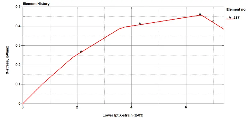
Fig-4

COMPARISON-

Now we have obtained the analytical results and the simulated results, by using an Excel sheet we can see the comparison by plotting a graph.

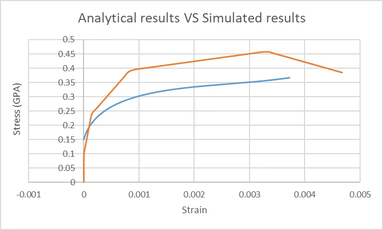
Fig-5

The True stress vs True strain from the simulation is compared with that of the original raw data. From the graph, we can say that our material model is up to the required accuracy as it almost matched the original raw data. This validates the created material using the raw data curve.

CONCLUSIONS:-

The main aim of the Week 9 challenge was to model a MAT 024 Piecewise Linear Plasticity material card from the given true stress/ strain raw data and use it to perform a uniaxial tension test of the given dog-bone specimen and also validate the post-processing stress-strain results with the given raw data. It was observed that the stress-strain curves obtained from the uniaxial test simulation almost behave in a similar fashion as the given raw data for the challenge.

LEARNING OUTPUT-

LEARNED HOW TO MODEL A MATERIAL CARD USING RAW DATA AND HOW WE CAN VALIDATE IT SUING THE SIMULATION DATA.