Week 9 Machining with Planer Challenge
Explicit Dynamics Analysis on Machining with Planer system
Objective
To perform an explicit dynamics simulation on Machining with Planer system in two Case Cutting Velocities, they are
Case 1: with a cutting velocity of 15000mm/s
Case 2: with a cutting velocity of 20000mm/s
To find out
- Equivalent Stress
- Total Deformation
- User defined temperature of body
Material data
Figure. 1 shows the Structural steel's properties in Ansys Workbench engineering data. It was used in the Machining with Planer system model's as Cutting tool material input. Figure. 2 shows the Steel 1006's properties in Ansys Workbench engineering data. It was used in the Machining with Planer system model's as Workpiece material input.
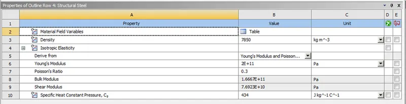
Figure. 1 Structural steel Engineering data.
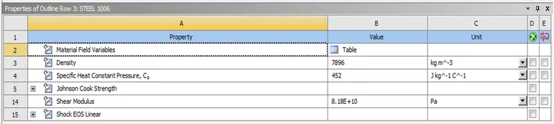
Figure. 2 Steel 1006 Engineering data.
Model Geomentry
Figure. 3 shows the imported given Machining with Planer system model in the mechanical modular.
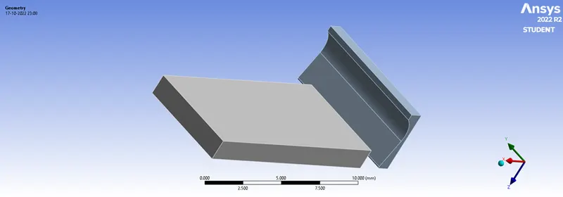
Figure. 3 Machining with Planer system model
Meshing
Figure. 4 illustrates the Patch conforming method of cutting tool, Figure. 5 illustrates the Edge sizing on four small edges of the workpiece with number of division 10 and Figure. 6 illustrates the model is Default meshed with no Adaptive sizing and high smoothing quality.
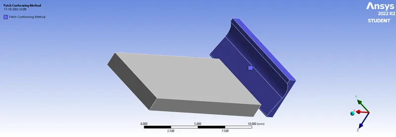
Figure. 4 Patch conforming method of cutting tool
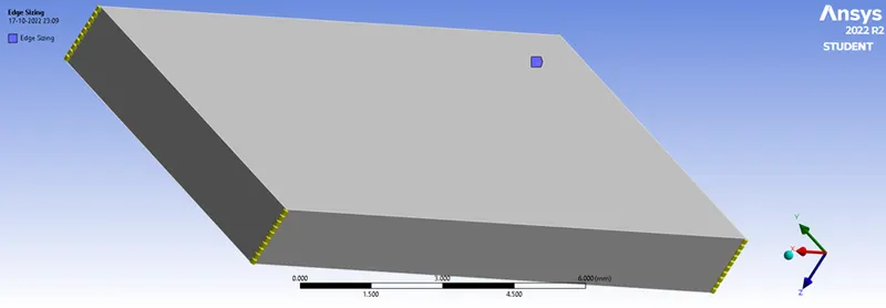
Figure. 5 Edge sizing of the workpiece
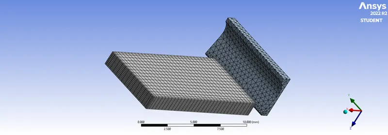
Figure. 6 Overall meshed model
Case 1
Velocity & Fixed joint
Figure. 7 illustrates the velocity joint on the Cuttingtool in the positive X-direction of globel co-rdinate system with a value of 15000 mm/s (as per case 1)and Figure. 8 illustrates the Fixed joint of the bottom face of the workpiece
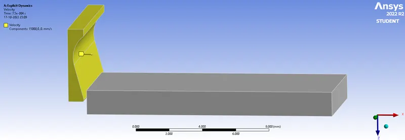
Figure. 7 Joint Velocity, Case 1.
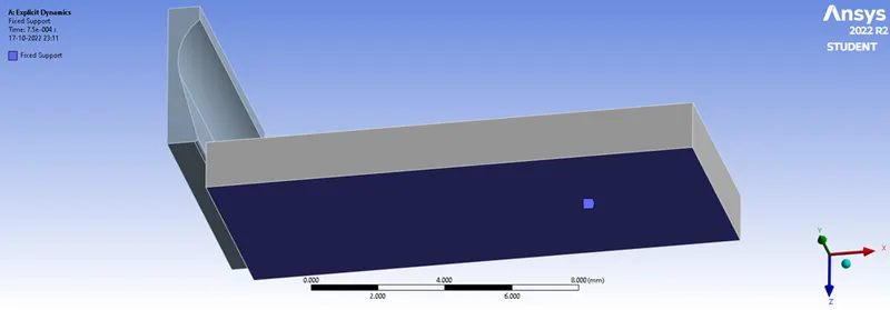
Figure. 8 Fixed Joint
Simulation Results
Total Deformation
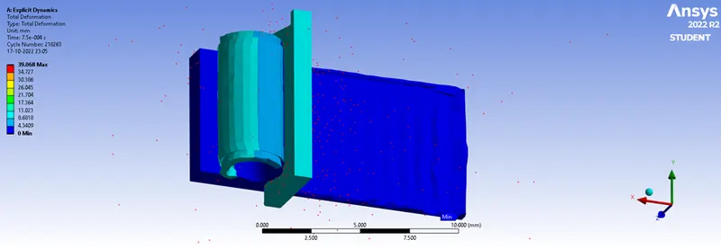
Figure. 9 Total Deformation with a cutting velocity of 15000mm/s
Equivalent Stress
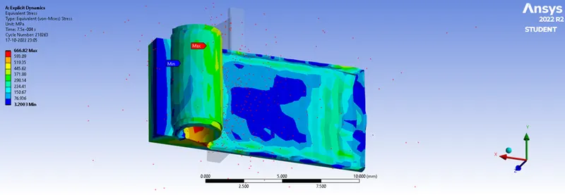
Figure. 10 Equivalent Stress with a cutting velocity of 15000mm/s
Temperature
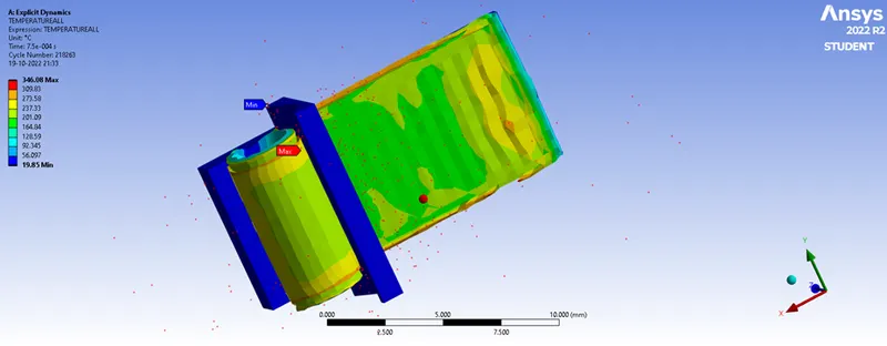
Figure. 11 Temperature with a cutting velocity of 15000mm/s
Case 2
Velocity & Fixed joint
Figure. 12 illustrates the velocity joint on the Cuttingtool in the positive X-direction of globel co-rdinate system with a value of 20000 mm/s (as per case 1)and Figure. 13 illustrates the Fixed joint of the bottom face of the workpiece
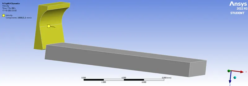
Figure. 12 Joint Velocity, Case 2.
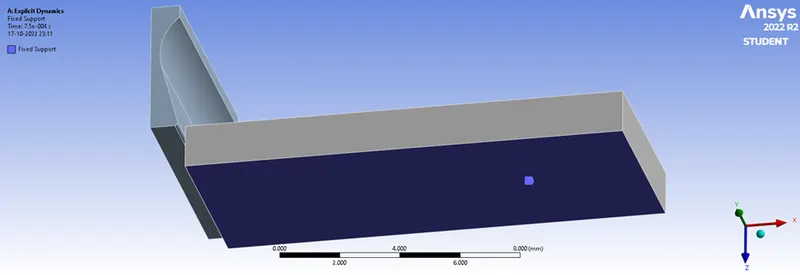
Figure. 13 Fixed Joint
Simulation Results
Total Deformation
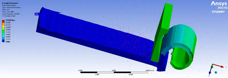
Figure. 14 Total Deformation with a cutting velocity of 20000mm/s
Equivalent Stress
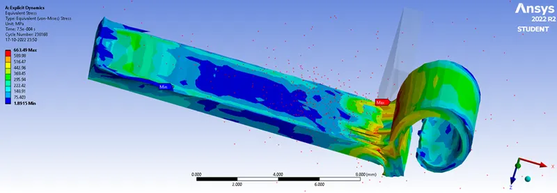
Figure. 15 Equivalent Stress with a cutting velocity of 20000mm/s
Temperature
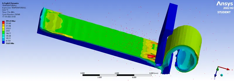
Figure. 16 Temperature with a cutting velocity of 20000mm/s
Comparision of Case 1 & Case 2
|
Parameters |
Case 1 |
Case 2 |
||
|
Maximum |
Minimum |
Maximum |
Minimum |
|
|
Total Deformation |
39.068 mm |
0 mm |
29.998 mm |
0 mm |
|
Equivalent Stress |
666.82 MPa |
3.2003 MPa |
663.49 MPa |
1.8915 MPa |
|
Temperature |
346.08 0C |
19.85 0C |
395.43 0C |
19.85 0C |
Conclusion
- Total deformation of Case 1 (15000mm/s) is higher than Case 2 (20000mm/s) and Similarly Equivalent Stress i higher in case 1.
- Temperature is higher in Case 2 compared to Case 1 and Case 2 has completely machined where as Case 1 is not
- From this comparison maching will have smooth and good surface finish in Case 2 hence it should be considered.