Week 9 - FVM Literature Review
Week 9 -
FVM Literature Review
Question :
What is Finite Volume Method(FVM), write down the major differences between FDM & FVM. Also, describe the need for interpolation schemes and flux limiters in FVM. You can use the 1D linear heat conduction equation as an example.
Aim :
Understand FVM, difference between FDM & FVM.
Theory :
There are various numerical method used to evaluate elliptic, parabolic or hyperbolic partial differential equations in the form of algebraic equations such as FVM, FDM, FEM and BEM.
These are methods for representing and evaluating partial differential equations in the form of algebraic equations.
FVM : Finite Volume Method
FDM : Finite Difference Method
FEM : Finite Element Method
BEM : Boundary Element Method
Finite Volume Method :-
Finite volume method is based on an unstructured (e.g. triangular) mesh. Therefore, it is suitable for irregular and complex geometries. FVM has another advantage over FEM for fluid mechanic problems. So far, the numerical methods that we presented have been based on PDEs. By contrast, FVM is based on the integral form of the conservation laws, rather than their differential form. This leads to more accuracy/stability, especially for sharp gradients (i.e. large derivatives) inside a domain, which is also called shock-capturing property. To explain this more clearly, as we mentioned before, the dynamics of flow can be described by conservation of mass, momentum, and energy. These conservation laws can be written as a system of PDEs. Alternatively, conservation laws can be expressed by integral equations (i.e. Reynolds transport theorem). For instance, the differential form of the continuity equation can be written as
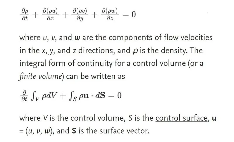
In the finite volume method, volume integrals in a partial differential equation that contain a divergence term are converted to surface integrals, using the divergence theorem. These terms are then evaluated as fluxes at the surfaces of each finite volume. Because the flux entering a given volume is identical to that leaving the adjacent volume, these methods are conservative. Another advantage of the finite volume method is that it is easily formulated to allow for unstructured meshes, therefore it is suitable for irregular and complex geometries.
The method is used in many computational fluid dynamics packages. "Finite volume" refers to the small volume surrounding each node point on a mesh.
FVM Methodology :
FVM is based on the integral form of the conservation laws, rather than their differential form. This leads to more accuracy/stability, especially for sharp gradients (i.e. large derivatives) inside a domain, which is also called shock-capturing property.
Furthermore, the FVM transforms the set of partial differential equations into a system of linear algebraic equations. Although the discrete approximation procedure in use in the FVM is distinctive, it also utilizes two basic steps.
Firstly, it transforms and integrates the PDEs into balance equations over an element. The process incorporates the changing of the surface and volume integrals into discrete algebraic relations over elements as well as their surfaces using an integration quadrature of a specified order of accuracy. This will result in a set of semi-discrete equations.
Secondly, in this next step, the interpolation profiles are chosen to estimate the variation of the variables within the element and relate the surface values of the variables to their cell values and thus transform the algebraic relations into algebraic equations. In regards to the two steps in the FVM process, your approximation selection affects the overall accuracy of the subsequent numeric.
Advantages and Disadvantages of FVM :
The FVM is a natural choice for solving CFD issues because the PDEs you have to resolve for CFD are conservation laws.
The FVM’s most significant advantage is that it only needs to do flux evaluation for the cell boundaries. Also, this is true for nonlinear issues as well, which, in turn, makes it an excellent choice for the handling of (nonlinear) conservation laws.
The accuracy of the FVM, for example, close to a corner of interest, can be increased by refining the mesh around that corner. However, the functions to estimate the solution is not easily made for higher-order. Therefore, this is a disadvantage of the FVM.
Example of Finite-volume method: CFD, heat transfer, and chemical engineering.
Finite Difference Method :-
The finite-difference method is the most direct approach to discretizing partial differential equations. You consider a point in space where you take the continuum representation of the equations and replace it with a set of discrete equations, called finite-difference equations. The finite-difference method is typically defined on a regular grid and this fact can be used for very efficient solution methods. The method is therefore not usually used for irregular CAD geometries, but more often for rectangular or block-shaped models.
Finite-Difference Method: Advantages and Disadvantages
The finite-difference method is defined dimension per dimension; this makes it easy to increase the “element order” to get higher-order accuracy. If you can fit the simulation in a rectangular or box-shaped geometry using a regular grid, efficient implementations are much easier than for finite-element and finite-volume methods. Regular grids are useful for very-large-scale simulations on supercomputers often used in, as mentioned before, meteorological, seismological, and astrophysical simulations.
Example of Finite-difference method: Weather calculations, astrophysics, seismology, physical realism in computer graphics, and special effects.
FVM Vs FDM
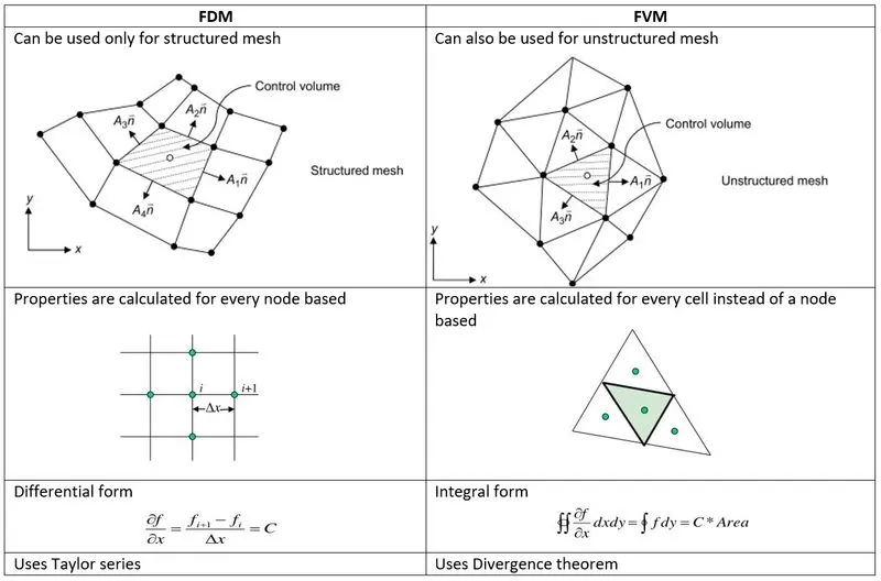
DIFFERENCES BETWEEN FDM AND FVM :
- Similar to the finite difference method or finite element method, values are calculated at discrete places on a meshed geometry.
- In finite difference, the dependent variable values are stored at the nodes But in finite volume method, the dependent values are stored in the centre of the finite volume.
- In FVM, conservation of mass, momentum, energy is ensured at each cell/finite volume level. This is not true in finite difference and finite element approach.
- One advantage of the finite volume method over finite difference methods is that it does not require a structured mesh (although a structured mesh can also be used).
- FDM is a differential scheme, that is approximation of a taylor series expansion. We try to write the first order, second order differential in terms of difference between two point values. This may bring in some approximation error.
- Finite Volume method is an integral scheme. Since you are integrating across the area, chance of error is minimized.
- Differential schemes are faster and error can be minimized if you have regular grids (squares and rectangles).
- Integral schemes are slightly slower but score over FDM when the mesh is irregular.
INTERPOLATION SCHEMES IN FINITE VOLUME METHOD:
The interpolation or the approximation schemes are required in the FVM method for the conversion of the integral form of the governing equation to an algebraic equation which can then be solved using various numerical methods. These schemes also play a significant role in the calculation of the values of the flow quantities in the point of concern from the values that are already known from their neighboring faces/cells. Some of the interpolation schemes are listed as follows:
- Upwind Interpolation
- Linear Interpolation
- Quadratic Upwind Interpolation Scheme(QUICK)
- Hybrid, TVD(Total variation dimension) & ENO(Essentially non-oscillatory) interpolation scheme.
1. Upwind Interpolation:
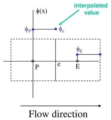
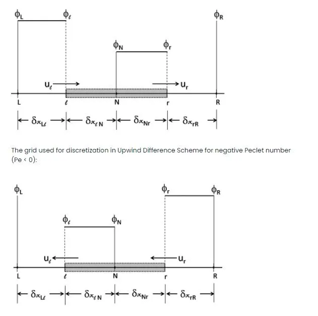
The upwind interpolation scheme is essentially used for convection-dominated problems. This interpolation scheme is essentially equivalent to using the forward difference method or backward difference method depending on the flow direction. Here, the direction of velocity at a given point determines the variable value to be used in an interpolation process. As the name suggests, we use the node upwind or upstream from the given node.
The upwind interpolation(UDS) for approximating the value of variable 'f' at the east face of the control volume is given by:
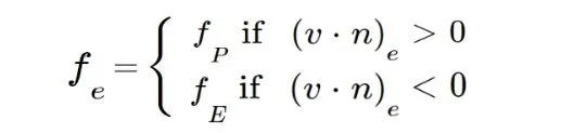
Upwind interpolation is the only approximation that satisfies the boundedness criterion unconditionally in the sense that irrespective of the velocity values and grid spacing, the solution will always remain bounded. This is the use of upwind interpolation which will never yield oscillatory solutions.
Upwind Interpolation is numerically diffusive. If we have sharp peaks or oscillatory values which are actually present in the solution then those would be damped out because of the presence of numerical diffusion and hence numerical diffusion is magnified in multi-dimensional flows, especially in cases where the flow is oblique to the grid space. Peaks or rapid variations in the variables will be smeared out because of the introduction of an additional diffusive coefficient which is called a numerical diffusive coefficient when UDS is used. It is first-order accurate and hence grids are required to obtain accurate solutions.
- Linear Interpolation(CDS):
The approximated value of the variable at control volume centroid by linear interpolation of the values at two nearest computational nodes.
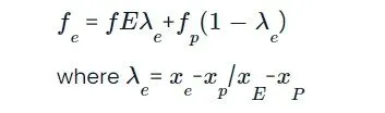
The linear interpolation is equivalent to the use of the CDS formula of the first-order derivative, and hence this scheme is also termed as Central Differencing Scheme(CDS).
This is 2nd-order accurate and may produce oscillatory results therefore small grids are preferred for this method. This is one of the most widely used interpolation methods.
- Quadratic Upwind Interpolation(QUICK):
The approximated values of the variable at the control volume's centroid by quadratic interpolation of the values at the three nearest computational nodes which consist of one downstream node 'D' and two upstream nodes 'UU'.
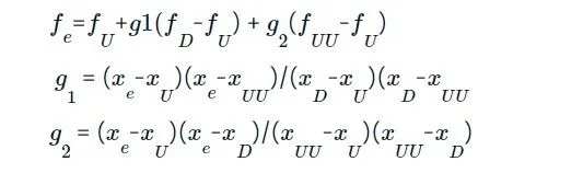
Quadratic Upwind Interpolation is third-order accurate in both uniform and non-uniform grids.
4 .Hybrid Interpolation scheme:
This interpolation method is a blend of both central differencing scheme and Upwind differencing scheme which is based on local peclet number. It can be described by the general partial equation as follows:
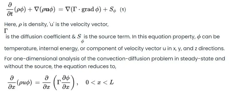
Here, Peclet number(Pe) is a non-dimensional parameter used as a measure of the relative strengths of convection and diffusion given as:
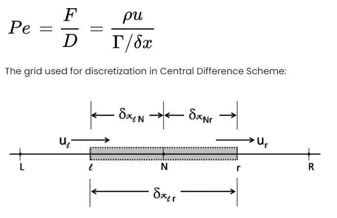
The grid used for discretization in Upwind Difference Scheme for positive Peclet number (Pe>0):
FLUX LIMITERS :
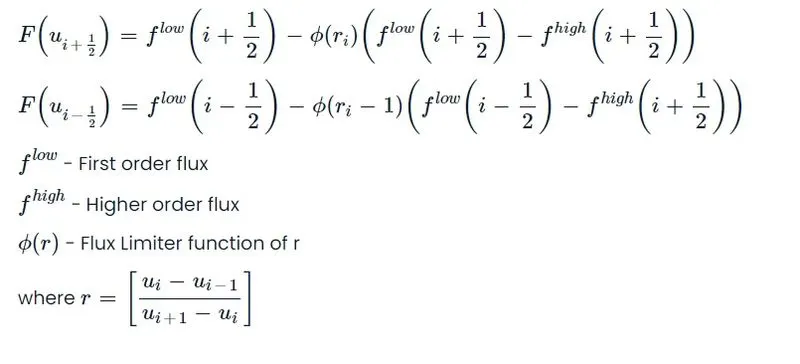
Flux limiters are used in high resolution schemes – numerical schemes used to solve problems in science and engineering, particularly fluid dynamics, described by partial differential equations (PDEs). They are used to avoid the spurious oscillations (wiggles) that would otherwise occur with high order spatial discretization schemes due to shocks, discontinuities or sharp changes in the solution domain. Use of flux limiters, together with an appropriate high resolution scheme, make the solutions total variation diminishing (TVD).
The main idea behind the construction of flux limiter schemes is to limit the spatial derivatives to realistic values – for scientific and engineering problems this usually means physically realisable and meaningful values.
Flux limiters are also referred to as slope limiters because they both have the same mathematical form, and both have the effect of limiting the solution gradient near shocks or discontinuities. In general, the term flux limiter is used when the limiter acts on system fluxes, and slope limiter is used when the limiter acts on system states (like pressure, velocity etc).
The limiter function is constrained to be greater than or equal to zero, i.e., ϕ(r)≥0
Therefore, when the limiter is equal to zero (sharp gradient, opposite slopes or zero gradient), the flux is represented by a low resolution scheme. Similarly, when the limiter is equal to 1 (smooth solution), it is represented by a high resolution scheme. The various limiters have differing switching characteristics and are selected according to the particular problem and solution scheme. No particular limiter has been found to work well for all problems, and a particular choice is usually made on a trial and error basis.
Flux limiters are used in numerical schemes to solve problems of highly coupled pde's. By intuition, one tends to use lower order numerical schemes for solving the p.d.e so that numerical oscillations are lower and doesn't involve unstable solutions or oscillations.
On the other hand, using higher order schemes comes up with computational cost and unnecessary computational power exploitation.
Hence, the motive behind the flux limiters is to limit the spatial derivatives near discontinuities so as to maintain the physical consistency of the problem. Highly applicable in the formation of shock blasts, sharp peaks presence.
Flux limiters are also referred to as slope limiters, since both are mathematically similar and physically limit the solution gradient near formation of shocks or any discontinuities
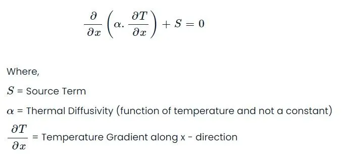
Discretization of 1D linear heat conduction equation using FVM –
In FDM, we have nodal points over which we solve the equations. Whereas in FVM, the points are the centres of the volumes, which stores the average quantities inside the volume.
For 1-D, we have the volumes as follows,
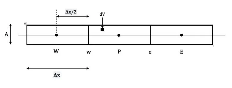
Considering control volume “P”, as shown in the above figure, surrounded by two control volumes E (east) and W (west) respectively. In our control volume, let us consider a very small volume “dV”. We solve our 1-D heat conduction equation in this volume dV and then we integrate it for the entire volume.
Therefore, the integral form of the governing equation is given by,
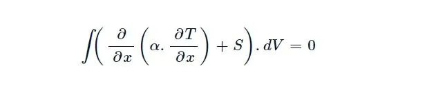
Therefore, we are taking the conservation equation that is valid at a single point and we are saying that, if it is valid at a single point, it is valid at the entire volume and that the properties of the system are conserved.
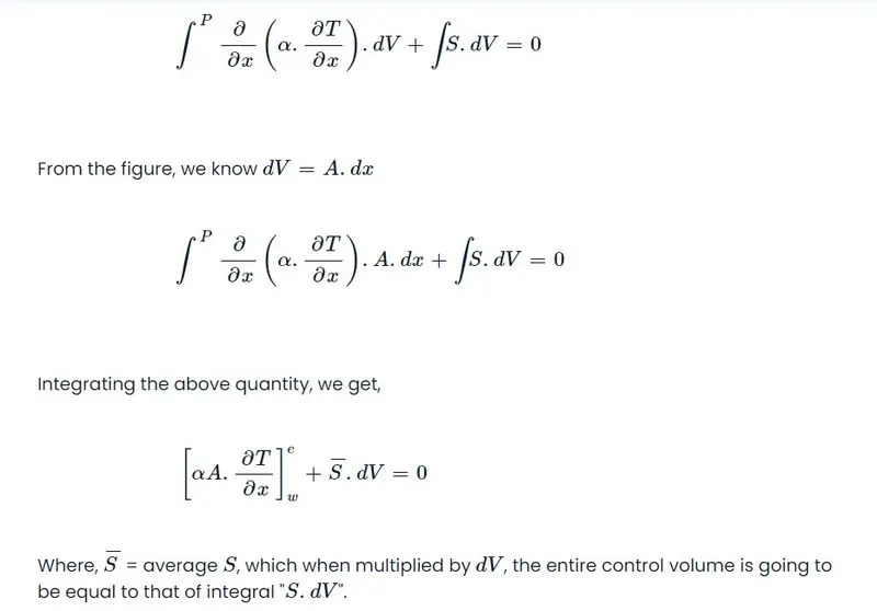
Therefore,
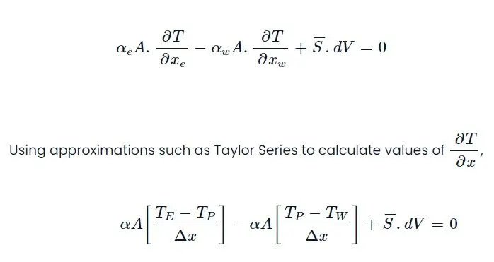
The above equation is in the form,
Heat flux In – Heat flux Out + Source Term = 0
How to choose an Interpolation function for a property?
Case I : Considering a linear interpolation function which is continuous inside the control volume but discontinous over the control surface
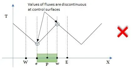
The below case clearly violates the heat flux conservation i.e., whatever amount of the heat flux enters inside the control volume through the control surface, the same amount of heat flux should leave the control volume through its outlet control surface assuming no heat generation inside the control volume which is the case that we have considered. (S =0)
Case II : Considering a linear interpolation function which is discontinuous inside the control volume at the grid or nodal point but continuous over the control surface
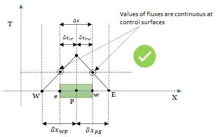
This case helps us give an insight of conserving the heat flux at the control surfaces by compromising the discontinuity inside the control volume, so that the conservation of flux is maintained at the control surface. Amount of flux entering the control surface at west end is equal to amount of flux leaving the control surface at east end. Hence this linear function can be useful for interpolating interface data of temperature between the control surface and grid point.
Reference: