Week 9 - FVM Literature Review

The Finite Volume Method:

The FVM(Finite Volume Method) other than the FDM(Finite Difference Method) is a Method we use to discretise the Governing Equations (Partial Differential Equations) into Algebraic Equations and to solve these Equations all over the Fluid Domain and thus solve the Fluid Flow. FDM and FVM discretise the PDEs by using completely different approach.

FVM is different from FDM

• In FVM we divide our Fluid Domain into large no. of smaller volumes or smaller Fluid Domains (Finite Volume) unlike grid points in case of FDM, we than discretise our Equations for these smaller volume and thus solve our Fluid Problem.
• In FVM the smaller fluid domain has their own inlet and outlet, since the Equations in these volumes are solved based on Conservation principles the law of conservation holds good for the complete Fluid Domain also this is due to the fact that in FVM the volume integral for the Equations are converted to surface integrals and evaluated as fluxes leaving or entering the control volume(the smaller volumes) since the entering and leaving flux are the same the properties are conserved.
• Before solving FVM we have to divide the Fluid Domain into smaller Volume, this process is called Meshing and its the most important part of the problem solving, it is a topic in it's own. One can choose where to have a Finer Mesh and where to have a Coarse Mesh or what type of Mesh to choose, etc. These all things affect the accuracy of the solution and the required computational resources.
• Every smaller volume is associated with a node which is located at the centroid of the volume, we calculate the value of Flow variable at these node points, for the points other than nodes we calculate the flow variables using Interpolation.
• There are various Interpolation Schemes we can use to solve for the flow variables these are

To name a few Interpolation schemes :

1. Linear Interpolation scheme
2. Upwind Interpolation scheme
3. Quadratic Upwind Interpolation scheme (QUICK scheme)
4. Hybrid Interpolation scheme
5. Total Variable Diminishing (TVD) Scheme.

Advantages of using Finite Volume Method over Finite Difference method

Solving Equations for Irregular Shaped Geometry by FVM

In case of FDM we have to find the approximations of the differential terms using the co-ordinate system we have, which means FDM works the best when we have a Fluid Domain where in we can create a grid aligned with the co-ordinate system, in simple words we need to simple geometry like a square or rectangular body, in order to create a grid pattern aligned with x-y coordinate.

If we want to solve for an irregular shaped body we need to use a method called as Variable transformation method. In this method we need to transform the co-ordinate variables into a different co-ordinate system which best align with the shape of the body so we could compute the differentials and after computation we need to again tranform it back to original coordinate system.

With FVM method we solve the integral equations directly for the finite volumes hence we need not need to approach a different goemetry by a completely different method, we just have to create a mesh and the generalise CFD code is enough to deal with any goemetry unlike developing a variable transformation math for every goemetry.

Since we can Generalise a lot of CFD problems using the FVM method it is the widely used Method by most of the CFD solver packages out there, even OpenFoam uses FVM in its Solver.

We use FDM since the method is very easy to code for simple goemetries and is therefore a good starting point to understand how to discretise and solve the PDEs.

Procedure for FVM Method:

Let us consider a general transport Equation with a property `phi` given as:

`(del(rhophi))/(delt)+"div"(rhophiu)="div"(Gamma"grad"(phi)) +S_(phi)`

Here `Gamma` is the Diffusion Coefficient ,`S_(phi)` is the Source term and `phi` is the dependent variable/property.

In this Equation we drop the transient and convective Part of the Equation to simplify it and we are left with Equation

`"div"(Gamma"grad"(phi)) +S_(phi)=0` -------------(A)

Simplifying Further let us consider only the 1-Dimensional Form of the Governing Equation

`(del)/(delx)(Gamma(delphi)/(delx))+S_(phi)=0`------------(B)

Next Step is to divide the domain into smaller volumes as shown in the figure below, we divide the volume into smaller volume with a node at the centre of every smaller volume.

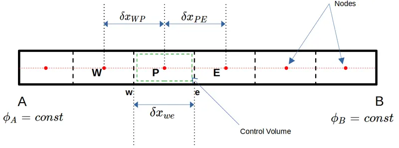
In the above Figure we have "A" and "B" as our boundary and value for `phi` for this boundary is given as boundary conditions

Further we integrate Equation (B) over the Control Volume (C.V)

`int_(CV)(del)/(delx)(Gamma(delphi)/(delx))dV+int_(CV)S_(phi)dV=0`

By Applying Gauss Divergence Theorem we have

`int_(CS)barn.[Gamma.(delphi)/(dx)]dA+int_(CV)S_(phi)dV = 0`

The First term in the above Equation is the Net Flux and is given by

`={[Gamma_e((delphi)/(delx))_eA_e]-[Gamma_w((delphi)/(delx))_wA_w]}`

So the Equation will be

`{[Gamma_e((delphi)/(delx))_eA_e]-[Gamma_w((delphi)/(delx))_wA_w]}+barS.DeltaV=0`----(C)

Now to Calculate `Gamma_e` ,`Gamma_w` , `((delphi)/(delx))_w` and `((delphi)/(delx))_e` We use the interpolation Techniques, Here we can use Linear Interpolation

`Gamma_e = (Gamma_P+Gamma_E)/2`

`Gamma_w = (Gamma_P+Gamma_W)/2`

`phi_w = (phi_W+phi_P)/2`

`phi_e = (phi_P+phi_E)/2`

Here we use the First order Approximations

`((delphi)/(delx))_w = (phi_P-phi_W)/(deltax_(wp)`

`((delphi)/(delx))_e = (phi_E-phi_P)/(deltax_(pe)`

Also if the source term is a function of a dependent variable than

`barSDeltaV = S_u+S_(p)phi_P`

Substituting the terms in the Equation (C) we get

`((Gamma_P+Gamma_E)/2)((phi_E-phi_P)/(deltax_(pe)))A_e -((Gamma_P+Gamma_W)/2)((phi_P-phi_W)/(deltax_(wp)))A_w+ S_u+S_(p)phi_P = 0`-----(D)

Further Simplifying this Equation we get

`[(Gamma_W+Gamma_P)/(2deltax_(wp))A_w+(Gamma_P+Gamma_E)/(2deltax_(pe))A_e+S_p]phi_P=((Gamma_P+Gamma_E)/(2deltax_(pe)))phi_EA_e+((Gamma_W+Gamma_P)/(2deltax_(wp)))phi_WA_w+S_u=0`----(E)

Now we have to apply Equation (E) to all the nodes and we will get a system of Linear Equations which we can solve using Matrix elimination method or even by using the Iterative Solver.

1. Linear Interpolation scheme

In this scheme we use a linear Interpolation to find the values at the faces of the control volume `phi_w` and `phi_e`

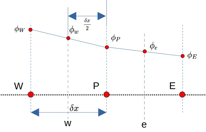
In the above Figure we can use the Equation of Line between "W" and "P" to find the value at "w"

`((deltax)/2-deltax)/(deltax)=(phi_w-phi_W)/(phi_W-phi_P)`

Simplifying this further we get

`(-phi_W+phi_P)/2=phi_w-phi_W`

`phi_w = (phi_W+phi_P)/2`

Similarly we can do the same for `phi_e`

`phi_e = (phi_P+phi_E)/2`

and the Derivatives can be calculated by central differencing approach

`((delphi)/(delx))_w = (phi_P-phi_W)/(deltax)`

`((delphi)/(delx))_e = (phi_E-phi_P)/(deltax)`

Depending upon the problem whether its a diffusion problem, convection problem or even a combined problem for Convection and Diffusion we use different Interpolation scheme which is well suited to the problem, in case of a diffusion problem Linear Interpolation scheme is well suited since it considers the values of both neighbouring points but the same is not true in case of a convection problem, in convection problem the flow/ direction of change in the property matters a lot, in that case depending upon the direction, the influence of the neighbouring points is different so hence in such case we use Upwind Interpolation scheme.

2. Upwind Interpolation Scheme

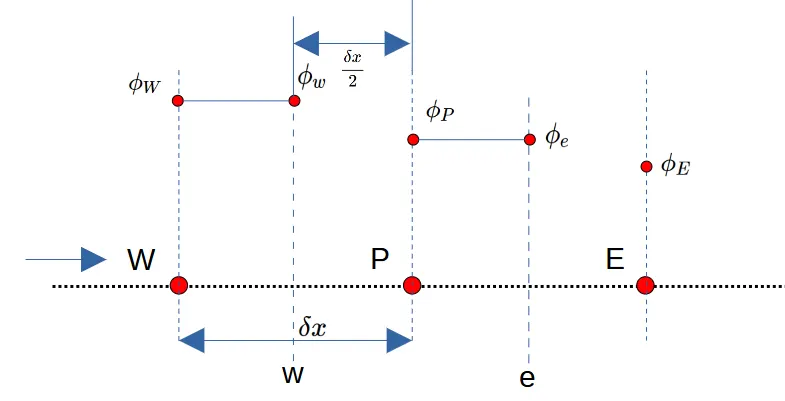
In First case we have the direction of the flow as left to right.

`phi_w = phi_W`

`phi_e = phi_P`

The derivatives can be evaluated by using Backward Difference scheme and Forward Difference Scheme

Backward Difference scheme is used when the flow is from left to right

and Forward Difference scheme is used when the flow is from right to left

`((delphi)/(delx))_w = (phi_P-phi_W)/(deltax_(wp)`

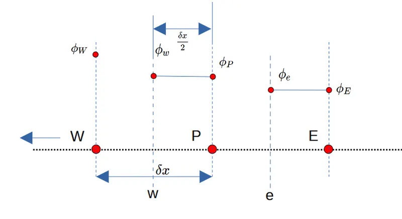
In the second case we have a flow from right to left

`phi_w = phi_P`

`phi_e = phi_E`

Collectively we can say that

`phi_w = {[phi_P if (barv.hatn>0)_w],[phi_W if (barv.hatn<0)_w]:}`

`phi_e = {[phi_E if (barv.hatn>0)_e],[phi_P if (barv.hatn<0)_e]:}`

Flux Limiters:

Generally when we use interpolation schemes in convective Equations the lower order schemes are stable but are dissipative in nature at discountinuities or sudden changing regions while the higher order methods are unstable and shows oscillations near the discontinuities or the areas of sudden change. We need the schemes which are stable and accurate these are named as high resolution schemes.

Flux Limiters are used when we want to maintain the higher order accuracy in the smooth regions and also retain the first order stability at the discontinuities or areas of sudden change.

`F(phi_w)=f^"low"(w)-alpha(r)[f^"low"(w)-f^"high"(w)]`

`F(phi_e)=f^"low"(e)-alpha(r)[f^"low"(e)-f^"high"(e)]`

`f^"low"` = flux with lower order accuracy

`f^"high"` = flux with higher order accuracy

`alpha(r) ` is the flux limiter function and `r = (phi_P-phi_W)/(phi_E-phi_P)`

This method is used to obtain high resolution results and used in TVD(Total Variable diminishing) scheme.