Week 5.1 - Mid term project - Solving the steady and unsteady 2D heat conduction problem
1. Solving Steady State Heat conduction Equation
The Steady State Heat conduction Equation in 2-D form is given as
`(del^2T)/(delx^2)+(del^2T)/(dely^2) = 0`-------------(1)
Where T = Temperature in (K) and x,y are the space co-ordinates
Now we need to discretise Equation (1), So we use Taylor's Table and appropriate numerical stencil to discretise the equation for second order approximation.
`(del^2T)/(delx^2) ~~(T_(i-1,j)-2T_(i,j)+T_(i+1,j))/(Deltax^2)`------(A)
`(del^2T)/(dely^2) ~~(T_(i,j-1)-2T_(i,j)+T_(i,j+1))/(Deltay^2)`------(B)
where i,j are the x and y indexes respectively
Adding Equation (A) and (B) we get
`(T_(i-1,j)-2T_(i,j)+T_(i+1,j))/(Deltax^2)+(T_(i,j-1)-2T_(i,j)+T_(i,j+1))/(Deltay^2)=0`
`(T_(i-1,j)-2T_(i,j)+T_(i+1,j))(Deltay^2)+(T_(i,j-1)-2T_(i,j)+T_(i,j+1))(Deltax^2)=0`
`T_(i,j) = (T_(i-1,j)*Deltay^2+T_(i+1,j)*Deltay^2+T_(i,j-1)*Deltax^2+T_(i,j+1)*Deltax^2)/(2(Deltay^2+Deltax^2))`------(C)
Since we consider a Rectangular Domain of same dimensions along X and Y axis we can further simplify Equation (C) since `Deltax = Deltay`
`T_(i,j) = (T_(i-1,j)+T_(i+1,j)+T_(i,j-1)+T_(i,j+1))/(4)`--------(D)
For Jacobi Method:
`T_(i,j)^(n+1) = (T_(i-1,j)^n+T_(i+1,j)^n+T_(i,j-1)^n+T_(i,j+1)^n)/(4)`-----(1)
For Gauss Siedel Method
`T_(i,j)^(n+1) = (T_(i-1,j)^(n+1)+T_(i+1,j)^n+T_(i,j-1)^(n+1)+T_(i,j+1)^n)/(4)`-----(2)
For Successive Relaxation Method
`T_(i,j)^(n+1) = (1-omega)T_(i,j)^n+(omega/4)(T_(i-1,j)^(n+1)+T_(i+1,j)^n+T_(i,j-1)^(n+1)+T_(i,j+1)^n)`------(3)
Note: Here (n+1) and (n) refers to latest and previous value of Iterations respectively.
Now we can solve Equations using Gauss Jacobi, Gauss Siedel or SOR Method and plot the Results as a contour plot
The MATLAB Code for the Steady State Heat Conduction is
% Solving Steady State Heat Conduction Equation
close all
clear
clc

% Defining Number of Intervals
Nx = 100;
Ny = 100;

% Number of grid points
nx = Nx+1;
ny = Ny+1;

% Rectangular Dimensions
Lx = 1;
Ly = 1;

% Grid spacing
dx = Lx/Nx;
dy = Ly/Ny;

x = (0:Nx)*dx;
y = (0:Ny)*dy;
[X,Y] = meshgrid(x,y);

% Convergence Criteria / Tolerance
eps = 1.e-4;

% Method Number
% 1 - Gauss Jacobi Method
% 2 - Gauss Siedel Method
% 3 - SOR Method using Gauss Siedel
method = 3;
if(method==1)
    type = 'Gauss Jacobi';
end
if(method==2)
    type = 'Gauss Siedel';
end
if(method==3)
    type = 'SOR method';
end


% Temperature value for the grid points
temp = zeros(nx,ny);


% Defining the Boundary Conditions Temperature in (K)
temp(:,ny) = 600;   % Top
temp(:,1)  = 900;   % Bottom
temp(1,:)  = 400;   % Left
temp(nx,:) = 800;   % Right
temp(1,1)   = (900+400)/2;
temp(1,ny)  = (600+400)/2;
temp(nx,1)  = (900+800)/2;
temp(nx,ny) = (600+800)/2;

% Solving with Iterative Method
temp_old = temp;    % Initial guess for the values of temperature
error = 2*eps;      % Error value at the beginning
ncount = 0;         % Iteration counter

while(error>eps)
    ncount = ncount + 1;
    for i = 2:nx-1
        for j = 2:ny-1
            if(method==1)
                % Solving by Gauss Jacobi Method
                temp(i,j) = (1/4)*(temp_old(i-1,j)+temp_old(i+1,j)...
                    +temp_old(i,j-1)+temp_old(i,j+1));
            end

            if(method==2)
                % Solving By Gauss Siedel Method
                temp(i,j) = (1/4)*(temp(i-1,j)+temp_old(i+1,j)...
                    +temp(i,j-1)+temp_old(i,j+1));
            end

            if(method==3)
                % SOR Method with Gauss Siedel method
                omega = 1.95;
                temp(i,j) = (1-omega)*temp_old(i,j)+ (omega/4)*(...
                    temp_old(i+1,j)+temp(i-1,j)+temp_old(i,j+1)+...
                    temp(i,j-1));
            end

        end
    end

    error = max(max(abs(temp(:,:)-temp_old(:,:))));

    if any(any(isinf(temp(:,:))) | any(isnan(temp(:,:))))
        % To check whether the Iterations are Diverging
        % If Diverging then stop the program
        fprintf("Iteration Diverged.!");
        return;
    end

    % Updating the pervious value of temperature
    temp_old = temp;

    % Displaying the Iteration count with the Error
    fprintf("\n%g - %e",ncount,error);

end
fprintf("\n Number of Iterations - %g",ncount);
% Plotting the countour plot
[c,h]=contourf(Y,X,temp(:,:),'ShowText','on');
c = colorbar;
colormap(jet);
c.FontSize = 11;
set(get(c,'label'),'string','Contour:Temperature(K)'...
    ,'FontSize',11);
xlabel('X(m)','Fontsize',14);
ylabel('Y(m)','Fontsize',14);
%h.LineColor = 'none';
%clabel(c,h);
title(sprintf('Steady State Heat Conduction over a Rectangular Domain \n No. of Iterations = %d, %s'...
    ,ncount,type));
The Results for the above code are as follows
a. Solving By Guass Jacobi Method we get:
Putting 'method = 1' in MATLAB Code
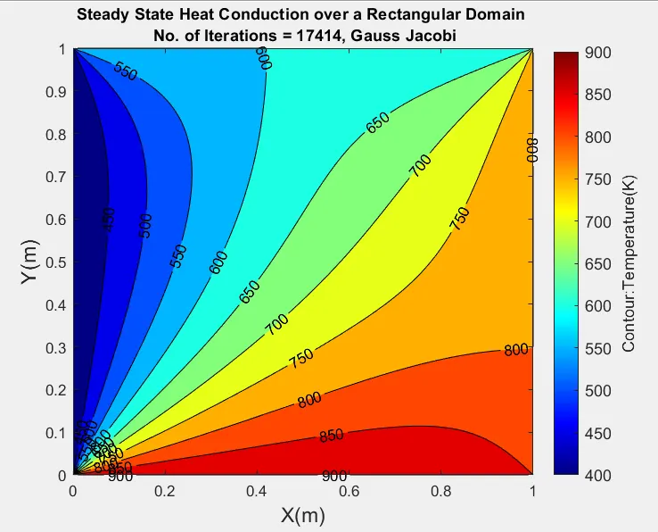
Conclusion: In Gauss Jacobi the convergence took 17414 number of Iterations for an error criteria of 1.e-4.
b.Solving by Gauss Siedel Method
Putting 'method = 2' in MATLAB Code
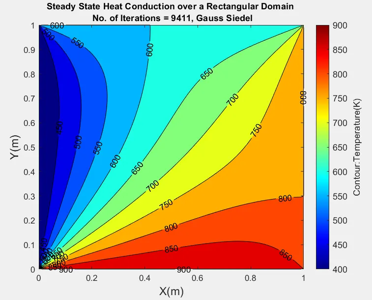
Conclusion: In case of Gauss Siedel Method the number of Iterations required to satisfy convergence criteria are 9411 which is far less than Gauss Jacobi Method, hence Gauss Siedel method converges faster than Gauss Jacobi Method.
c. SOR(Successive Over Relaxation) Method
Putting 'method = 3' in MATLAB Code
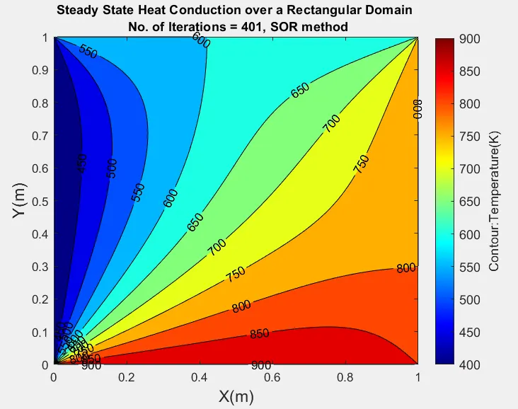
Conclusion: By adjusting the value of `omega`(Relaxation Factor) and setting it as overlaxed, we can obtain convergence in just 401 iterations, here we used `omega = 1.95`, but we also need to be careful that if we keep on increasing the value of Relaxation Factor beyond cartain value the Iterations will diverge.
Now by Solving Steady state heat conduction by Iterative Method we conclude that Gauss Siedel Method converges more quickly than Gauss Jacobi Method. The convergence rate of SOR Method can be controlled by changing the relaxation factor, one can choose over relaxed method by changing lambda to be greater than 1, in which case the system tends to converge more rapidly but depending upon the equations in play the iterations may diverge if a high relaxation factor is used, conversely if the equations in play are non linear equations than the iterations may diverge even with Gauss Jacobi or Gauss Siedel method, in that case we have to use the SOR method and set the relaxation factor less than 1, the convergence may take time and more iterations but the results are bound to converge even if the equations are non Linear equations.
In our case the Equations are all Linear Equations and we solve the Heat conduction Equations by using relaxation factor as `omega = 1.95`, and by doing this the convergence happens more rapidly and takes the least iterations than the Gauss Jacobi or Siedel Method.
2. Solving Unsteady State Heat Conduction Equation
a. Solving using Explicit Scheme
The PDE for unsteady state Heat Conduction Equation is Given by
`(delT)/(delt) = alpha((del^2T)/(delx^2)+(del^2T)/(dely^2))`------(A)
Now we need to discretise Equation (A) in order to solve it as a system of Algebric Equations
First we solve the Equation by using a Explicit Scheme
We need the first order approximation of the time derivative of Temperature since we use only present time and previous time step (only 2 grid points are involved on time grid)
`(delT)/(delt) ~~ (T_(i,j)^(n+1)-T_(i,j)^n)/(Deltat)`------(1)
Similiarly we take the second order approximation for the Space Derivative
`(del^2T)/(delx^2) ~~(T_(i-1,j)^n-2T_(i,j)^n+T_(i+1,j)^n)/(Deltax^2)`------(2)
`(del^2T)/(dely^2) ~~(T_(i,j-1)^n-2T_(i,j)^n+T_(i,j+1)^n)/(Deltay^2)`------(3)
Putting (1)(2)(3) in equation (A) we get
`(T_(i,j)^(n+1)-T_(i,j)^n)/(Deltat)=alpha((T_(i-1,j)^n-2T_(i,j)^n+T_(i+1,j)^n)/(Deltax^2)+(T_(i,j-1)^n-2T_(i,j)^n+T_(i,j+1)^n)/(Deltay^2))`------(B)
And since we use a symetric Rectangular Dimensions `Deltax = Deltay=h`
Simplifying Equation (B) Further we get
`T_(i,j)^(n+1)=T_(i,j)^n+(alpha*DeltaT)/(h^2)(T_(i-1,j)^n-2T_(i,j)^n+T_(i+1,j)^n)+(T_(i,j-1)^n-2T_(i,j)^n+T_(i,j+1)^n)`
- Here since it is a explicit scheme for stability we have CFL criteria
- Here the CFL number is given as CFL = `(2*alpha*DeltaT)/(h^2)`
- For a stable solution the CFL < 0.5, so the boundary line for stability is CFL = 0.5, from this we get a value for time step as `Deltat = (CFL*h^2)/(2*alpha)`
- We use the following value for `Deltat` in our MATLAB Code
Note: Here (n+1) and (n) refers to latest and previous timesteps respectively.
The MATLAB Code is as follows
% Usteady State Heat conduction by Explicit method
clear
clc
close all

% Defining Number of Intervals
Nx = 20;
Ny = 20;

%Defining the number of time steps
nt = 2000;

%Defining Diffusivity Constant
alpha = 1.4;


% Number of grid points
nx = Nx+1;
ny = Ny+1;

% Rectangular Dimensions
Lx = 1;
Ly = 1;

% Grid spacing
dx = Lx/Nx;
dy = Ly/Ny;

% Defining dt by the CFL criteria for explicit method
% CFL = (2*alpha*dt)/(dx^2)
% CFL < 0.5 for stability
CFL = 0.5;
dt = (CFL*dx^2)/(2*alpha);

%dt = 0.0002;
D = alpha*dt/(dx^2);

x = (0:Nx)*dx;
y = (0:Ny)*dy;
[X,Y] = meshgrid(x,y);

% Error criteria
eps = 1.e-4;

% Initial value for the temperature
temp =300*zeros(nx,ny,nt);

% Defining the Boundary Conditions Temperature in (K)
temp(:,ny,:) = 600;   % Top
temp(:,1,:)  = 900;   % Bottom
temp(1,:,:)  = 400;   % Left
temp(nx,:,:) = 800;   % Right
temp(1,1,:)   = (900+400)/2;
temp(1,ny,:)  = (600+400)/2;
temp(nx,1,:)  = (900+800)/2;
temp(nx,ny,:) = (600+800)/2;

temp_old = temp(:,:,1);

% Solving by Explicit method
for t = 1:nt
    for i = 2:nx-1
        for j = 2:ny-1
            % Solving by Explicit Method
            temp(i,j,t+1)=(1-4*D)*temp_old(i,j)+...
                D*(temp_old(i-1,j)+temp_old(i+1,j)+temp_old(i,j-1)+temp_old(i,j+1));
        end
    end
    temp_old = temp(:,:,t);
end

% Plotting the results by a countour plot
i = 0;
time = 0;
for t = 1:10:nt-1
    i = i + 1;
    % Plotting the countour plot
    [c,h]=contourf(Y,X,temp(:,:,t),'ShowText','on');
    c = colorbar;
    colormap(jet);
    c.FontSize = 11;
    set(get(c,'label'),'string','Contour:Temperature(K)'...
        ,'FontSize',11);
    xlabel('X(m)','Fontsize',14);
    ylabel('Y(m)','Fontsize',14);
    title(sprintf("Unsteady State Heat Conduction(Explicit) \n Time - %f sec ",time));
    %h.LineColor = 'none';
    %clabel(c,h);
    pause(0.003);
    M(i) = getframe(gcf);
    time = dt+dt*(t-1);
    if(max(max(abs(temp(:,:,t)-temp(:,:,t+1))))<eps)
        % This means that system has reached a Steady State
        break;
    end

end

%Creating a Video File with decreased Frame Rate for the animation
videofile = VideoWriter('Unsteady_state_heat_conduction_explicit.avi','Uncompressed AVI');
videofile.FrameRate = 9;
open(videofile);
writeVideo(videofile,M);
close(videofile);
The Results for the Following MATLAB Code are
Conclusions:
- The Explicit Method doesn't require a convergence loop to be solved, So we solve this method directly without using any iterative solver.
- The Explicit Method do require a Stability Criteria i.e CFL number to be less than or equal to 0.5, if this number increases than the Solution becomes unstable and gives us unbounded results.
- The Steady State is achieved at time = 0.84 sec.
b. Solving using Implicit Scheme
For the case of Implicit Method the Equation (B) changes as follows
`(T_(i,j)^(n+1)-T_(i,j)^n)/(Deltat)=alpha((T_(i-1,j)^(n+1)-2T_(i,j)^(n+1)+T_(i+1,j)^(n+1))/(Deltax^2)+(T_(i,j-1)^(n+1)-2T_(i,j)^(n+1)+T_(i,j+1)^(n+1))/(Deltay^2))`------(B')
`Deltax = Deltay = h` Since we are using a equal sized rectangular Domain
This we further simplify the Equation as follows
`T_(i,j)^(n+1)=(1)/(1-(4alphaDeltat)/(h^2))(T_(i,j)^n+(Deltat*alpha)/(h^2)(T_(i-1,j)^(n+1)+T_(i+1,j)^(n+1)+T_(i,j-1)^(n+1)+T_(i,j+1)^(n+1)))`-----------(C)
Putting `(Deltat*alpha)/(h^2) = D`
We implement Equation (C) for Solving in Implicit Scheme
For Gauss Jacobi Method
`T_(i,j)^(n+1,"new") = (1)/(1-4D)(T_(i,j)^n+D(T_(i-1,j)^(n+1,"old")+T_(i+1,j)^(n+1,"old")+T_(i,j-1)^(n+1,"old")+T_(i,j+1)^(n+1,"old")))`--------(1)
For Gauss Siedel Method
`T_(i,j)^(n+1,"new") = (1)/(1-4D)(T_(i,j)^n+D(T_(i-1,j)^(n+1,"new")+T_(i+1,j)^(n+1,"old")+T_(i,j-1)^(n+1,"new")+T_(i,j+1)^(n+1,"old")))`---------(2)
For SOR Method we have
`T_(i,j)^(n+1,"new") = (1-omega)T_(i,j)^(n+1,"old")+omega(1/(1+4D)*(T_(i,j)^(n)+D(T_(i-1,j)^(n+1,"new")+T_(i+1,j)^(n+1,"old")+T_(i,j-1)^(n+1,"new")+T_(i,j+1)^(n+1,"old"))))`-------(2)
Note: Here "new" and "old" refers to latest and previous Iteration values of temperature respectively.
The MATLAB Code is
% Unsteady State heat conduction Equation
clear
clc
close all

% Defining Number of Intervals
Nx = 100;
Ny = 100;

%Defining the number of time steps
nt = 500;

%Defining Diffusivity Constant
alpha = 1.4;


% Number of grid points
nx = Nx+1;
ny = Ny+1;

% Rectangular Dimensions
Lx = 1;
Ly = 1;

% Grid spacing
dx = Lx/Nx;
dy = Ly/Ny;

% No Stability criteria for an Implicit method
% Implicit Methods are inherentily Stable
dt = 1.e-3;
D = alpha*dt/(dx^2);

x = (0:Nx)*dx;
y = (0:Ny)*dy;
[X,Y] = meshgrid(x,y);

% Convergence Criteria / Tolerance
eps = 1.e-4;

% Method Number
% 1 - Gauss Jacobi Method
% 2 - Gauss Siedel Method
% 3 - SOR Method using Gauss Siedel
method = 3;
if(method==1)
    type = 'Gauss Jacobi';
end
if(method==2)
    type = 'Gauss Siedel';
end
if(method==3)
    type = 'SOR method';
end

%Iterative Method
temp = zeros(nx,ny,nt);

% Defining the Boundary Conditions Temperature in (K)
temp(:,ny,:) = 600;   % Top
temp(:,1,:)  = 900;   % Bottom
temp(1,:,:)  = 400;   % Left
temp(nx,:,:) = 800;   % Right

% Solving by Implicit Scheme
for t=2:nt
    error = 2;
    temp(:,:,t)=temp(:,:,t-1);
    temp_old = temp(:,:,t);
    ncount = 0;
    while(error > eps)
        ncount = ncount + 1;
        for i = 2:nx-1
            for j = 2:ny-1
                if(method==1)
                    %Gauss Jacobi Method
                    temp(i,j,t)= (1/(1+4*D))*(temp(i,j,t-1)+(D)*(temp_old(i-1,j)...
                       +temp_old(i+1,j)+temp_old(i,j-1)+temp_old(i,j+1)));
                end
                if(method==2)
                    %Gauss Siedel Method
                    temp(i,j,t)= (1/(1+4*D))*(temp(i,j,t-1)+(D)*(temp(i-1,j,t)...
                       +temp_old(i+1,j)+temp(i,j-1,t)+temp_old(i,j+1)));
                end
                if(method==3)
                    % SOR Method
                    omega  = 1.85;
                    DT = temp(i-1,j,t)+temp_old(i+1,j)+temp(i,j-1,t)+temp_old(i,j+1);
                    temp(i,j,t)=(1-omega)*temp_old(i,j)+(omega/(1+4*D))*(temp(i,j,t-1)+D*(DT));
                    %temp(i,j,t) = (1/(1-omega*(1+4*D)))*(temp_old(i,j)+omega*(temp(i,j,t-1)+(D)*(temp(i-1,j,t)...
                       %+temp_old(i+1,j)+temp(i,j-1,t)+temp_old(i,j+1))));
                end

            end
        end
        error = max(max(abs(temp(:,:,t)-temp_old)));
        if any(any(isinf(temp(:,:,t))) | any(isnan(temp(:,:,t))))
            fprintf("Iterations Diverged.!");
            return;
        end
        temp_old = temp(:,:,t);
        fprintf('%g - %e\n',ncount,error);
    end
    fprintf('\n%g\n',ncount);
    Iterations(t-1) = ncount;
end

% Plotting the results by a countour plot
time = 0;
i = 0;
for t = 1:4:nt-1
     i = i + 1;
    % Plotting the countour plot
    [C,h]=contourf(Y,X,temp(:,:,t),'ShowText','on');
    c = colorbar;
    colormap(jet);
    c.FontSize = 11;
    clabel(C,h,'LabelSpacing',150);
    set(get(c,'label'),'string','Contour:Temperature(K)'...
        ,'FontSize',11);
    xlabel('X(m)','Fontsize',14);
    ylabel('Y(m)','Fontsize',14);
    title(sprintf("Unsteady State Heat Conduction- %s \n Time = %f sec ",type,time));
    %h.LineColor = 'none';
    %clabel(c,h);
    pause(0.003);
    M(i) = getframe(gcf);
    time = dt+dt*(t-1);
    if(max(max(abs(temp(:,:,t)-temp(:,:,t+1))))<eps)
        % This means that system has reached a Steady State
        break;
    end

end
fprintf("Average Number of Iterations per time steps = %g\n",round(mean(Iterations)));

%Creating a Video File with decreased Frame Rate for the animation
videofile = VideoWriter('Unsteady_state_heat_conduction_Implicit.avi','Uncompressed AVI');
videofile.FrameRate = 9;
open(videofile);
writeVideo(videofile,M);
close(videofile);
The Results for this Code are
a.By Gauss Jacobi Method
Conclusion:
- Average Number of Iterations per time steps = 157
b.By Gauss Siedel Method
Conclusions:
- Guass Siedel method converges more faster than Guass Jacobi Method
- Average Number of Iterations per time step - 92
c. By SOR(Successive Over Relaxation) Method
here we have used a Over Relaxed System with `omega = 1.85`
Conclusions:
- In case of SOR Method with relaxation Factor `omega = 1.85` the system converges with very fewer Iterations than Gauss Siedel or Gauss Jacobi Method
- The Number of Iterations taken on an average per time step is 34.
- We have to carefully select the relaxation factor since if we increase the relaxation factor than the Iterations will Diverge.