Week 12 - Validation studies of Symmetry BC vs Wedge BC in OpenFOAM vs Analytical H.P equation
Problem Statement: Comparing the Velocity profiles of a Laminar Viscous Flow through a pipe for Wedge BC and Symmetry BC with the Analytical Results obtained by Solving Hagen-Poiseuille's Equations.
The Reynolds Number for the Flow is given by Re = 2100
The Hagen Poiseuille's Equation for solving velocity profile are given as
`r(dp)/(dx) = mu(d)/(dr)(r(du)/(dr))`
The velocity profile is given as :
`R^2/(4mu)((dp)/(dx))[1-(r^2)/(R^2)]`
`R = D/2`
`V_"avg" = R^2/(4mu)(dp)/(dx)`
`V_"max" = 2V_"avg"`
`(dp)/(dx)=(8muV_"avg")/(R^2)`
`DeltaP = (8muLV_"avg")/(R^2)`
`DeltaP` is the pressure drop along the Length of the pipe
The shear stress variation can be
`tau = (4muV_"avg".r)/(R^2)`
The Maximum shear stress occurs at the walls of the pipe
Now from the Reynold's Number we can calculate the average velocity `V_"avg"`
`Re = (rho.V_"avg".D)/(mu)`
`u(r) = 2V_"avg"[1-(r^2)/(R^2)]`
`tau(r) = (4muV_"avg".r)/(R^2)`
Diameter of the Pipe is assume to be D =60 mm
The viscocity of the Fluid(water) is given as
`mu = 1.0016" x "10^-3 " "(Ns)/m^2`
The Density of Water is given as
`rho = 997 " "(kg)/m^3`
Hence the Kinematic Viscocity (`nu`) is given as `nu = mu/rho`
`nu = 1.0046" x "10^-6" "m^2/s`
The Hydrodynamic Entrance Length is given by an Empirical Relation
`L_e = 0.06*Re*D`
We consider the Length of the pipe slightly greater than the Entrance Length
We create a MATLAB Code to generate 'blockMeshDict' for our case
% Solving for Hagen Pousielle's Flow
clc
clear
close all

% Solving for Hagen Pousielle's Flow
% We assume a Reynold's Number of Re = 2100
Re = 2100;
% and Diameter of the Pipe is assume as
D   = 0.006;         % Diameter of Pipe in (m)
mu  = 1.0016e-3;     % Viscosity of Water (Pa.s) at 20 deg Celcius
rho = 997;           % Density of water (kg/m^3) at 20 deg Celcius
L = Re*D*0.06+1.8 ; % Length of the pipe in (m)
%L = 0.02;
R = D/2;             % Radius of pipe

% Calculating the Average Velocity by using Re = (rho.V.D)/(mu)
Vavg = Re*mu/(rho*D);       % Average velocity
Vmax = 2*Vavg;              % Maximum Velocity
DP = 8*mu*L*Vavg/(R^2);     % Pressure Variation
KDP = DP/rho;               % Kinematic Pressure (m^2/s^2)
nu = mu/rho;                % Kinematic Viscosity
% Calculating the Vertices of the fluid Element
theta = 10;      % Angle of wedge in (deg)

x0 = 0;
y0 = 0;
z0 = 0;

x1 = 0;
y1 = R*cosd(theta/2);
z1 = -R*sind(theta/2);

x2 = 0;
y2 = y1;
z2 = -z1;

x3 = L;
y3 = 0;
z3 = 0;

x4 = L;
y4 = y1;
z4 = z1;

x5 = L;
y5 = y2;
z5 = z2;

f1 = fopen('blockMeshDict','w');

% The headers
h1 = '/*--------------------------------*- C++ -*----------------------------------*\';
h2 = '  =========                 |';
h3 = '  \\      /  F ield         | OpenFOAM: The Open Source CFD Toolbox';
h4 = '   \\    /   O peration     | Website:  https://openfoam.org';
h5 = '    \\  /    A nd           | Version:  9';
h6 = '     \\/     M anipulation  |';
h7 = '\*---------------------------------------------------------------------------*/';
h8 = '// * * * * * * * * * * * * * * * * * * * * * * * * * * * * * * * * * * * * * //';

fprintf(f1,'%s\n',h1);
fprintf(f1,'%s\n',h2);
fprintf(f1,'%s\n',h3);
fprintf(f1,'%s\n',h4);
fprintf(f1,'%s\n',h5);
fprintf(f1,'%s\n',h6);
fprintf(f1,'%s\n',h7);
fprintf(f1,'//theta = %d deg\n\n',theta);
fprintf(f1,'%s\n','FoamFile');
fprintf(f1,'%s\n','{');
fprintf(f1,'\t%s\t%s\n','format','ascii;');
fprintf(f1,'\t%s\t%s\n','class','dictionary;');
fprintf(f1,'\t%s\t%s\n','object','blockMeshDict;');
fprintf(f1,'%s\n','}');
fprintf(f1,'%s\n\n',h8);
fprintf(f1,'%s\n\n','convertToMeters 1;');
fprintf(f1,'%s\n','vertices');
fprintf(f1,'%s\n','(');

fprintf(f1,'\t(%0.8f %0.8f %0.8f)\n',x0,y0,z0);
fprintf(f1,'\t(%0.8f %0.8f %0.8f)\n',x1,y1,z1);
fprintf(f1,'\t(%0.8f %0.8f %0.8f)\n',x2,y2,z2);
fprintf(f1,'\t(%0.8f %0.8f %0.8f)\n',x3,y3,z3);
fprintf(f1,'\t(%0.8f %0.8f %0.8f)\n',x4,y4,z4);
fprintf(f1,'\t(%0.8f %0.8f %0.8f)\n',x5,y5,z5);

fprintf(f1,'%s\n\n',');');

fprintf(f1,'blocks\n');
fprintf(f1,'(\n');
fprintf(f1,'\thex (2 5 3 0 1 4 3 0) (240 12 5) simpleGrading (30 10 1)\n');
fprintf(f1,');\n\n');

fprintf(f1,'edges\n');
fprintf(f1,'(\n');
%fprintf(f1,'\tarc 1 2 %d (1 0 0)\n',theta);
%fprintf(f1,'\tarc 4 5 %d (1 0 0)\n',theta);
fprintf(f1,'\tarc 1 2 (%0.8f %0.8f %0.8f)\n',0,R,0);
fprintf(f1,'\tarc 4 5 (%0.8f %0.8f %0.8f)\n',L,R,0);
%fprintf(f1,'\tspline 1 2 \n\t(\n\t\t(%0.8f %0.8f %0.8f)\n\t\t(%0.8f %0.8f %0.8f)\n\t)\n',...
%    0,R*sind(90-theta/4),R*cosd(90-theta/4),0,R*sind(90-theta/4),-R*cosd(90-theta/4));
%fprintf(f1,'\tspline 4 5 \n\t(\n\t\t(%0.8f %0.8f %0.8f)\n\t\t(%0.8f %0.8f %0.8f)\n\t)\n'...
%    ,L,R*sind(90-theta/4),R*cosd(90-theta/4),L,R*sind(90-theta/4),-R*cosd(90-theta/4));
fprintf(f1,');\n\n');

fprintf(f1,'boundary\n');
fprintf(f1,'(\n');

fprintf(f1,'\tinlet\n');
fprintf(f1,'\t{\n');
fprintf(f1,'\t\ttype patch;\n');
fprintf(f1,'\t\tfaces\n');
fprintf(f1,'\t\t(\n');
fprintf(f1,'\t\t\t(0 1 2 0)\n');
fprintf(f1,'\t\t);\n');
fprintf(f1,'\t}\n\n');

fprintf(f1,'\toutlet\n');
fprintf(f1,'\t{\n');
fprintf(f1,'\t\ttype patch;\n');
fprintf(f1,'\t\tfaces\n');
fprintf(f1,'\t\t(\n');
fprintf(f1,'\t\t\t(3 5 4 3)\n');
fprintf(f1,'\t\t);\n');
fprintf(f1,'\t}\n\n');

fprintf(f1,'\tfixedWall\n');
fprintf(f1,'\t{\n');
fprintf(f1,'\t\ttype wall;\n');
fprintf(f1,'\t\tfaces\n');
fprintf(f1,'\t\t(\n');
fprintf(f1,'\t\t\t(2 1 4 5)\n');
fprintf(f1,'\t\t);\n');
fprintf(f1,'\t}\n\n');

fprintf(f1,'\tfront\n');
fprintf(f1,'\t{\n');
fprintf(f1,'\t\ttype wedge;\n');
fprintf(f1,'\t\tfaces\n');
fprintf(f1,'\t\t(\n');
fprintf(f1,'\t\t\t(1 0 3 4)\n');
fprintf(f1,'\t\t);\n');
fprintf(f1,'\t}\n\n');

fprintf(f1,'\tback\n');
fprintf(f1,'\t{\n');
fprintf(f1,'\t\ttype wedge;\n');
fprintf(f1,'\t\tfaces\n');
fprintf(f1,'\t\t(\n');
fprintf(f1,'\t\t\t(2 5 3 0)\n');
fprintf(f1,'\t\t);\n');
fprintf(f1,'\t}\n\n');

fprintf(f1,'\taxis\n');
fprintf(f1,'\t{\n');
fprintf(f1,'\t\ttype empty;\n');
fprintf(f1,'\t\tfaces\n');
fprintf(f1,'\t\t(\n');
fprintf(f1,'\t\t\t(0 3 3 0 )\n');
fprintf(f1,'\t\t);\n');
fprintf(f1,'\t}\n\n');

fprintf(f1,');\n\n');

fprintf(f1,'mergePatchPairs\n');
fprintf(f1,'(\n');
fprintf(f1,');\n\n');

fprintf(f1,'%s\n',h8);
fclose(f1);

Vavg
nu
KDP
This is the "blockMeshDict" file for `theta = 10deg` and "wedge" Boundary condition
Similiarly we have to create "blockMeshDict" for 25deg and 45deg for both wedge BC and symmetry BC
/*--------------------------------*- C++ -*----------------------------------*\
  =========                 |
  \\      /  F ield         | OpenFOAM: The Open Source CFD Toolbox
   \\    /   O peration     | Website:  https://openfoam.org
    \\  /    A nd           | Version:  9
     \\/     M anipulation  |
\*---------------------------------------------------------------------------*/
//theta = 45 deg

FoamFile
{
	format	ascii;
	class	dictionary;
	object	blockMeshDict;
}
// * * * * * * * * * * * * * * * * * * * * * * * * * * * * * * * * * * * * * //

convertToMeters 1;

vertices
(
	(0.00000000 0.00000000 0.00000000)
	(0.00000000 0.00277164 -0.00114805)
	(0.00000000 0.00277164 0.00114805)
	(2.55600000 0.00000000 0.00000000)
	(2.55600000 0.00277164 -0.00114805)
	(2.55600000 0.00277164 0.00114805)
);

blocks
(
	hex (2 5 3 0 1 4 3 0) (240 12 1) simpleGrading (30 10 1)
);

edges
(
	arc 1 2 (0.00000000 0.00300000 0.00000000)
	arc 4 5 (2.55600000 0.00300000 0.00000000)
);

boundary
(
	inlet
	{
		type patch;
		faces
		(
			(0 1 2 0)
		);
	}

	outlet
	{
		type patch;
		faces
		(
			(3 5 4 3)
		);
	}

	fixedWall
	{
		type wall;
		faces
		(
			(2 1 4 5)
		);
	}

	front
	{
		type wedge;
		faces
		(
			(1 0 3 4)
		);
	}

	back
	{
		type wedge;
		faces
		(
			(2 5 3 0)
		);
	}

	axis
	{
		type empty;
		faces
		(
			(0 3 3 0 )
		);
	}

);

mergePatchPairs
(
);

// * * * * * * * * * * * * * * * * * * * * * * * * * * * * * * * * * * * * * //
Similarily we need to update the initial condition the Velocity and Pressure at initial time step the "controlDict" and the "transportproperties"
For Initial inlet Velocity we have to input our `V_avg` calculated by using Reynolds number `V_"avg"=0.3516 m/s`
/*--------------------------------*- C++ -*----------------------------------*\
  =========                 |
  \\      /  F ield         | OpenFOAM: The Open Source CFD Toolbox
   \\    /   O peration     | Website:  https://openfoam.org
    \\  /    A nd           | Version:  9
     \\/     M anipulation  |
\*---------------------------------------------------------------------------*/
FoamFile
{
    format      ascii;
    class       volVectorField;
    object      U;
}
// * * * * * * * * * * * * * * * * * * * * * * * * * * * * * * * * * * * * * //

dimensions      [0 1 -1 0 0 0 0];

internalField   uniform (0 0 0);

boundaryField
{
    inlet
    {
        type            fixedValue;
        value           uniform (0.3516 0 0);
    }

    outlet
    {
    	type		zeroGradient;
    }

    axis
    {
    	type		empty;
    }

    fixedWall
    {
        type            noSlip;
    }

    front
    {
        type            wedge;
    }

    back
    {
    	type  		 wedge;

    }

}

// ************************************************************************* //
Next we need to update our outlet pressure since our pipe is open to atmosphere we give the Pressure (The Kinematic Pressure) as `P_atm/rho` which is approximately " 1.0073"
/*--------------------------------*- C++ -*----------------------------------*\
  =========                 |
  \\      /  F ield         | OpenFOAM: The Open Source CFD Toolbox
   \\    /   O peration     | Website:  https://openfoam.org
    \\  /    A nd           | Version:  9
     \\/     M anipulation  |
\*---------------------------------------------------------------------------*/
FoamFile
{
    format      ascii;
    class       volScalarField;
    object      p;
}
// * * * * * * * * * * * * * * * * * * * * * * * * * * * * * * * * * * * * * //

dimensions      [0 2 -2 0 0 0 0];

internalField   uniform 0;

boundaryField
{
    inlet
    {
        type            zeroGradient;
    }

    outlet
    {
        type            fixedValue;
        value           uniform 1.0073;
    }

    fixedWall
    {
        type            zeroGradient;
    }

    axis
    {
    	type 		empty;
    }

    front
    {
        type            wedge;
    }

    back
    {
        type            wedge;
    }
}

// ************************************************************************* //
Next we need to update the Kinematic viscosity `nu` in our transportproperties
/*--------------------------------*- C++ -*----------------------------------*\
  =========                 |
  \\      /  F ield         | OpenFOAM: The Open Source CFD Toolbox
   \\    /   O peration     | Website:  https://openfoam.org
    \\  /    A nd           | Version:  9
     \\/     M anipulation  |
\*---------------------------------------------------------------------------*/
FoamFile
{
    format      ascii;
    class       dictionary;
    location    "constant";
    object      transportProperties;
}
// * * * * * * * * * * * * * * * * * * * * * * * * * * * * * * * * * * * * * //

nu              [0 2 -1 0 0 0 0] 1.00316e-6;


// ************************************************************************* //
Here since the flow is an incompressible viscous Laminar flow we are going to use "icoFoam" as our solver
Next we need to update "controlDict", also we need to select our timestep so that the stability criteria (CFL Number) is satisfied
/*--------------------------------*- C++ -*----------------------------------*\
  =========                 |
  \\      /  F ield         | OpenFOAM: The Open Source CFD Toolbox
   \\    /   O peration     | Website:  https://openfoam.org
    \\  /    A nd           | Version:  9
     \\/     M anipulation  |
\*---------------------------------------------------------------------------*/
FoamFile
{
    format      ascii;
    class       dictionary;
    location    "system";
    object      controlDict;
}
// * * * * * * * * * * * * * * * * * * * * * * * * * * * * * * * * * * * * * //

application     icoFoam;

startFrom       startTime;

startTime       0;

stopAt          endTime;

endTime         1.7;

deltaT          0.00025;

writeControl    timeStep;

writeInterval   20;

purgeWrite      0;

writeFormat     ascii;

writePrecision  6;

writeCompression off;

timeFormat      general;

timePrecision   6;

runTimeModifiable true;


// ************************************************************************* //
After updating the above files in the case folder we need to run the "blockMesh" command
The Mesh will be generated in the case folder as "polymesh"
Next we need to solve the Iteration by command "icoFoam"
After the case is completed we need to export the Results which includes
1. Variation of Pressure and Velocity along the length of the pipe
2. Velocity Profiles at different positions along the length of the pipe
We than analyse this Results in the MATLAB
clear
clc
close all

% Solving for Hagen Pousielle's Flow
% We assume a Reynold's Number of Re = 2100
Re = 2100;
% and Diameter of the Pipe is assume as
D   = 0.006;         % Diameter of Pipe in (m)
mu  = 1.0016e-3;     % Viscosity of Water (Pa.s) at 20 deg Celcius
rho = 997;           % Density of water (kg/m^3) at 20 deg Celcius
L = Re*D*0.06+1.8 ; % Length of the pipe in (m)
Ra = D/2;             % Radius of pipe

% Calculating the Average Velocity by using Re = (rho.V.D)/(mu)
Vavg = Re*mu/(rho*D);       % Average velocity
Vmax = 2*Vavg;              % Maximum Velocity
DP = 8*mu*L*Vavg/(Ra^2);     % Pressure Variation

% Exported File
% We Extract the data in MATLAB Variable SOL
aa = {'L(0.001).csv','L(0.1).csv','L(0.5).csv','L(1.5).csv'};
bb = {'10_HP','25_HP','45_HP','10S_HP','25S_HP','45S_HP'};
% SOL = {L,R,UaL,PaL,U_0.001,U_0.1,U_0.5,U_1.5}
index = [5 6 7 8];
folder = 'C:\Users\ksth5\Desktop\Engineering Career\PROJECTS\MATLAB\CFD_MATLAB\Flow_Through a Pipe\';
SOL = zeros(202,8,6);
sol_data = zeros(7,4);
for gg = 1:6
    for hh = 1:4
        filename = strcat(folder,bb{gg},'\',aa{hh});
        f1 = fopen(filename,'r');
        tline = fgetl(f1);
        n = 1;
        while 1
            tline = fgetl(f1);
            if ~ischar(tline)
                break
            end
            %disp(tline)
            l = 1;
            h = 1;
            for j = 1:length(tline)
                if(tline(j)==',')
                    a(n,l) = str2double(tline(h:j-1));
                    l = l+1;
                    h = j+1;
                end

            end
            n = n+1;
        end
        fclose(f1);
        SOL(:,2,gg) = [a(:,6);-flip(a(:,6))]; % r
        SOL(:,index(hh),gg) = [a(:,1);flip(a(:,1))]; %U
    end
    f1 = fopen(strcat(folder,bb{gg},'\','PU_L.csv'));
    tline = fgetl(f1);
    n = 1;
    while 1
        tline = fgetl(f1);
        if ~ischar(tline)
            break
        end
        %disp(tline)
        l = 1;
        h = 1;
        for j = 1:length(tline)
            if(tline(j)==',')
                a(n,l) = str2double(tline(h:j-1));
                l = l+1;
                h = j+1;
            end

        end
        n = n+1;
    end
    fclose(f1);
    SOL(1:101,1,gg) =a(:,6); % l
    SOL(1:101,3,gg) =a(:,4); % P
    SOL(1:101,4,gg) =a(:,1); % U
end

% Plotting our Results
titl = {'10deg Wedge','25deg Wedge','45deg Wedge','10deg Symmetry',...
    '25deg Symmetry','45deg Symmetry'};
figure(1)
for j = 1:6
    subplot(2,3,j)
    U = SOL(1:101,4,j);
    LEN = SOL(1:101,1,j);
    plot(LEN,U,'b','Linewidth',1.1);
    hold on
    for kl = 2:length(LEN)
        DUDL(kl) = (U(kl-1)-U(kl))/(LEN(kl-1)-LEN(kl));
        if (DUDL(kl)<=1e-2)
            break;
        end
    end
    plot(LEN(kl),U(kl),'ko','Linewidth',1.2);
    hold on
    plot([LEN(kl) LEN(kl)],[U(kl) 0],'k:','Linewidth',0.9);
    Le = LEN(kl);
    textdata = strcat('Le = ',num2str(Le));
    text(0.8,0.3,textdata);
    grid minor
    xlabel('Length(m)');
    ylabel('Velocity(m/s)');
    title(titl{j});
    sgtitle(strcat('Comparing the Value for Hydrodynamic Entrance Length Le = '...
        ,num2str(L-1.8)));
    sol_data(j+1,4) = Le;
end

% Comparing our Results with the Analytical Equation

% Velocity Profile of a fully developed laminar Flow
r = linspace(Ra,0,100);
u = 2.*Vavg.*(1-(r.^2)./(Ra.^2));
u = [u,flip(u)];
r = [r,-flip(r)];

figure(2);
for j = 1:6
    subplot(2,3,j);
    plot(u,r,'r','Linewidth',1.1);
    hold on
    U = SOL(:,8,j);
    R = SOL(:,2,j);
    plot(U(1:5:end),R(1:5:end),'b+','Linewidth',1.1);
    xlabel('Radial Distance(m)');
    ylabel('Velocity (m)');
    title(titl{j});
    sol_data(j+1,1)=max(U);
    sgtitle('Velocity Profile at L = 1.5 m');

end

%Shear stress profile
figure(3)
for j = 1:6
    subplot(2,3,j)
    tau = sign(r).*(4.*mu.*Vavg.*r)./(Ra^2);
    plot(tau,r,'r','Linewidth',1.1);
    tau_wall = max(tau);
    hold on
    U = SOL(:,8,j);
    R = SOL(:,2,j);
    TAU = zeros(length(R),1);
    % Shear Stress profile for exported data
    for i = 2:length(R)
        TAU(i) = mu*((U(i-1)-U(i))./(R(i)-R(i-1)));
    end
    TAU = (sign(R).*TAU);
    plot(TAU(1:4:end),R(1:4:end),'b+','Linewidth',1.1);
    ylabel('r(m)');
    xlabel('Shear Stress(N/m^2)');
    title(titl{j});
    sgtitle('Shear Stress Profile at L = 1.5 m');
    sol_data(j+1,2) = max(TAU);
end

%Pressure Profile
figure(4)
for j = 1:6
    subplot(2,3,j);
    % Considering the Pressure in (Pa)
    P = SOL(1:101,3,j).*rho;
    LEN = SOL(1:101,1,j);
    plot(LEN,P,'b','Linewidth',1.1);
    hold on
    DPr = P(end)-P(1);
    textdata = strcat('DP ',num2str(DPr));
    text(1,1800,textdata);
    grid minor
    xlabel('Length(m)');
    ylabel('Pressure(Pa)');
    title(titl{j});
    sgtitle('Pressure Variation along Length');
    sol_data(j+1,3)=DPr;
end

% Calculating the parameters
% U_max , Tau_max , DP , Le
sol_data(1,1) = Vmax;
sol_data(1,2) = tau_wall;
sol_data(1,4) = L-1.8;
sol_data(1,3) = DP;

% Output
fprintf("---------------------------------------------------\n");
fprintf("|%9s|%9s|%9s|%9s|%9s|\n",'type','u_max','tau_max','DP','Le');
fprintf("---------------------------------------------------\n");
type = {'HP','10deg W','25deg W','45deg W','10deg S','25deg S','45deg S'};
for i = 1:7
    fprintf("|%9s|%5.7f|%5.7f|%6.4f|%5.6f|\n",type{i},sol_data(i,1),sol_data(i,2),sol_data(i,3),sol_data(i,4));
    fprintf("---------------------------------------------------\n");

end
The Results for the above code are given as
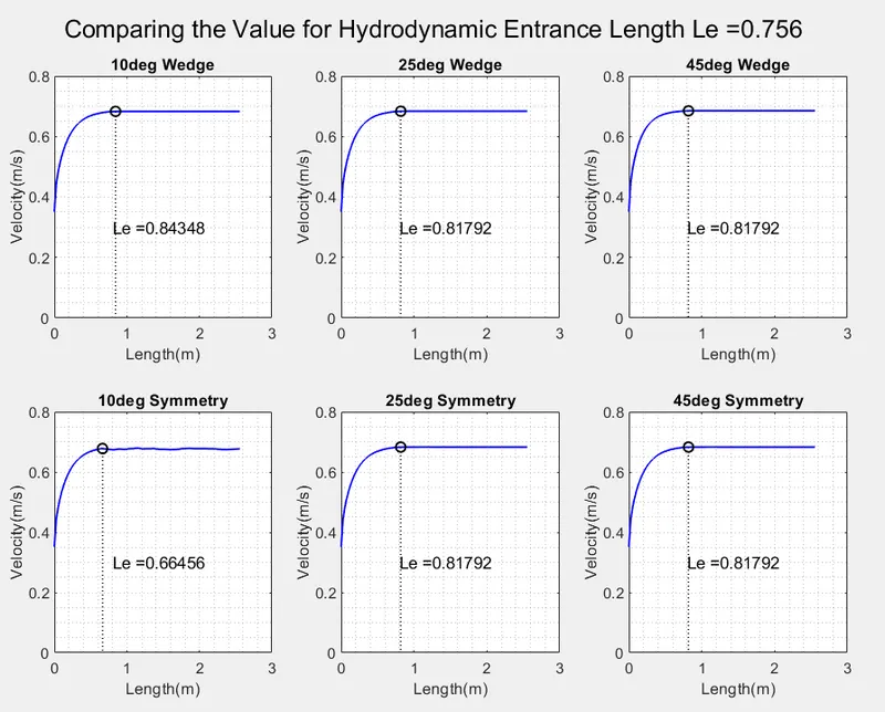
1. Validating The Hydrodynamic Entrance Length
The following plot compares the variation of Velocity along the Length of the pipe, The Length at which Velocity no longer changes with respect to the Length is called as the Hydrodynamic Entrance Length. By the Empirical Formula as mentioned above the Le = 0.756 and Le for various cases are as follows.
2. Validating the Fully Developed Flow with the Analytical profile
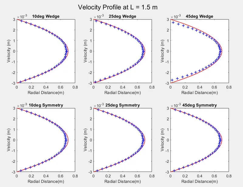
The plot below shows the velocity profile at L = 1.5 m for different cases which is in blue color and these profiles are compared with the Analytical Profile which is in red color
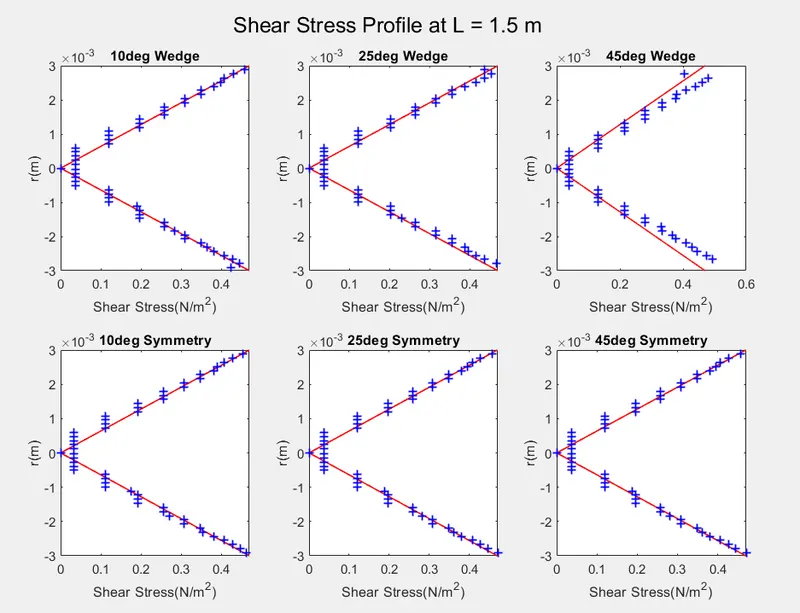
3.Validating the Shear stress profile of the cases with that of the analytical profile
The shear stress profile at L = 1.5 m is given below which is compared with the analytical profile in Red
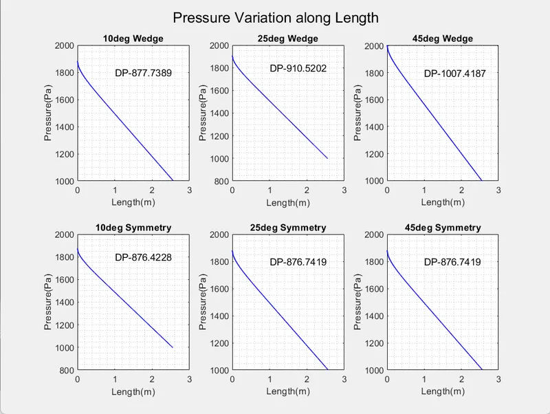
4. Validating the pressure drop
The Pressure drop across the length of the pipe is given as follows ,its in (-ve) sign since the pressure is decreasing as we go along length due to friction loss.
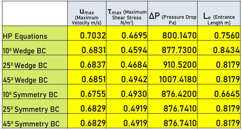
We further compare the Analytical values of Maximum velocity, shear stress , pressure drop and Hydrodynamic Entrance Length
Conclusion:
From the above Results we can conclude that for the Wedge Boundary conditions as the angle increases from 10deg to 45deg the results become less and less accurate in the above table it can be seen how the maximum values are drifting away as we increase the wedge angle from 10 deg to 45 deg
Where as when we compare the results of symmetry boundary conditions, the results are stable even if we increase the value of the angle from 10 deg to 45 deg, quite interestingly the results tend to be more accurate when we increase the angle.