Week 8 - Simulation of a backward facing step in OpenFOAM
Problem Statement:
To Simulate the incompressible-Laminar Viscous Flow of a Fluid through a Backward facing Step Geometry. We have to do it as per the Following Cases
Case 1: Simulation of Flow without using any grading Factor (i.e G.F = 1)
Case 2: Simulation of Flow with G.F = 0.2 and the cell should be finer near the walls,
Mesh specification
- Number of cells along the x direction (longer dimension) = 200
- Number of cells along the longer y direction = 20
Fluid Domain and the Boundary Conditions:
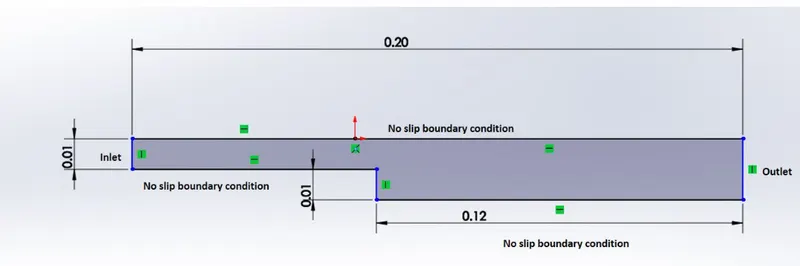
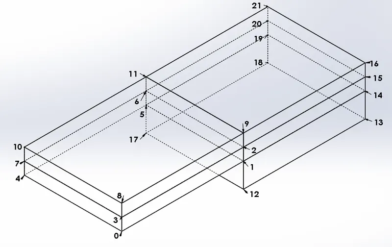
We set up our case as per the given boundary condition and the Fluid Domain, before Formulating the Case, we need to divided the Fluid Domain into Suitable Blocks for the purpose of Meshing, since we also have to follow the Mesh Regulations specified above that is we need to have a finer mesh near the walls, therefore such type of Mesh grading is possible when we divide the Fluid Domain into 5 blocks as given below
(FIG-1)
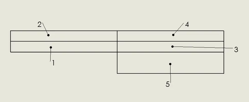
here we divided Blocks as 1 and 2 for the mesh grading along Y axis and blocks 4 and 3 are divided to maintain consistency for the overall solution
Starting with the Case:
- We look into OpenFoam tutorials and search a similar case in the tutorial folder.
- Then we need to copy this case file to our OpenFoam run directory, (OpenFoam provides a run directory where all you cases can run, we do this to avoid any change in the tutorial files provided by OpenFoam)
- We need to find which solver can solve for our Case, this depends upon the Flow physics and conditions.
- We need to use the blockMesh utility provided by OpenFoam to create a Mesh file, this can be done by updating our Geometry (Faces, Points, edges, etc) in the file named as "blockMeshDict" and run the command "blockMesh"
- We have to change our Initial conditions and the time interval ,time step ,etc since this is a Transient Simulation.
- Finally we need to run the calculation using a Appropriate Solver and post process the results in "ParaView".
OpenFoam is operated via Command Line Interface/ from the Terminal
We can go to Terminal Window and type the commands to navigate through the OpenFoam workspace.
Step 1.
Enter command "tut" to enter in the OpenFoam Tutorial Folder
List the contents in the folder with "l" and enter the folder incompressible by entering command "cd incompressible"
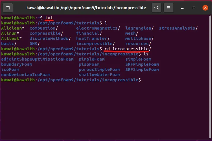
Since our aim is to simulate a incompressible laminar Viscous flow we enter folder incompressible
Then we need to go inside the folder "icoFoam" since this solver solves the incompressible Laminar flow Equation which is the most basic equation,
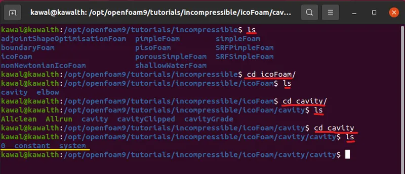
Here we go to icoFoam/cavity, here "cavity" is the case we need we can take any case and modify it as per our need, but we choose cavity in this case, to avoid confusion with the external mesh file present in the "elbow" folder.
Step 2:
In this step we copy the cavity folder to our dedicated run folder
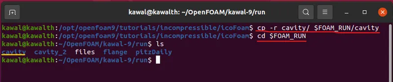
here command: "cp -r cavity/ $FOAM_RUN/cavity" copies complete folder cavity to the run folder, where we can run the simulation
Further we also list the folders inside the run folder and we can see "cavity" over there.
Step 3:
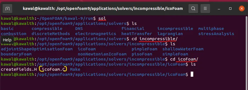
we can type the command "sol" on our terminal window, this will take us to the Solvers folder of the installation, here we can navigate through different solvers and select the one which represents our Fluid Physics, for us we go to "incompressible" and than into "icoFoam", this would be our prefered solver, we can further inspect the .C file of the solver.
Step 4:
Here we need to set-up the mesh file using the blockMesh utility
To setup the Geometry in the "blockMeshDict" we need to number the vertices of our blocks of the Fluid Domain, we then need to define the mesh type for the blocks and finally we need to define the condition at each faces like inlet, outlet or fixed wall
We can navigate to the file "blockMeshDict" by using command
gedit cavity/cavity/cavity/system/blockMeshDict

Understanding the file "blockMeshDict":
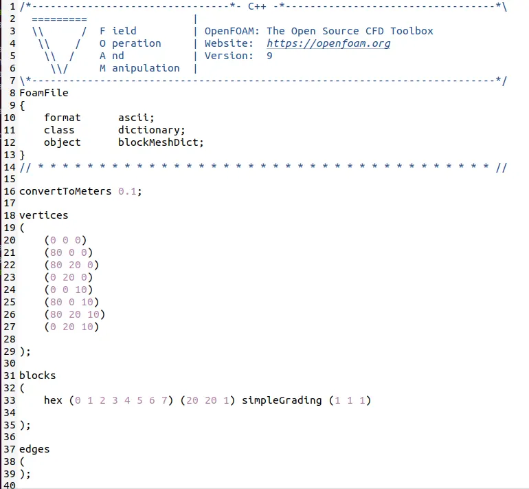
FoamFile : It identifies that the file is an OpenFoam file, object is "blockMeshDict"
convertToMeters : This value is a scaling factor used to convert the size into meter, for eg if we are specifying the sizes in "meter" than value of "convertToMeters" = 1, if the sizes are specified in "mm" than the value for "convertToMeters" = 0.001
vertices: This specifies the points for the geometry.
blocks: In this we define the blocks, type of mesh we want, and what should be the grading scale along the X,Y and Z axis
here they have defined "hex(0 1 2 3 4 5 6 7) (20 20 1) simpleGrading (1 1 1)"
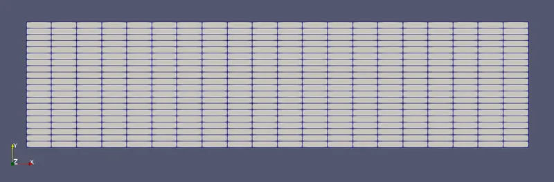
this means that we have to built a block with face(0 1 2 3) and face(4 5 6 7) which has 20 cells along X axis and 20 cells along Y axis and only 1 along Z axis, and Grading means controlling the density of the cells
for eg. if we had "hex(0 1 2 3 4 5 6 7) (20 20 1) simpleGrading (1 1 1)" then the mesh would look like
and now if we add a G.F along X-axis "hex(0 1 2 3 4 5 6 7) (20 20 1) simpleGrading (0.1 1 1)" then the mesh would have looked like
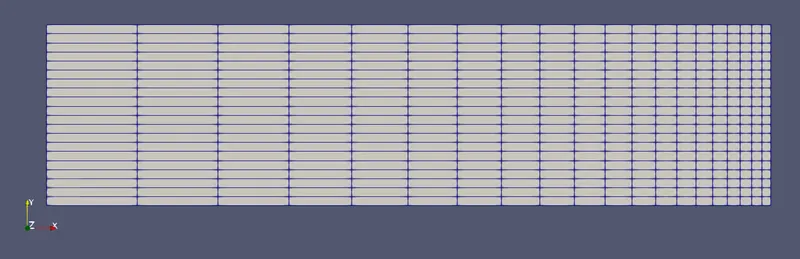
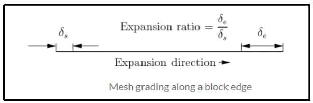
The Grading Factor allows the user to refine and grade the mesh along a specific direction. The ratio (G.F) is that of the width of the end cell along one edge of the block to the width of the start cell along the edges as shown below
The same thing can be applied along Y and Z axis
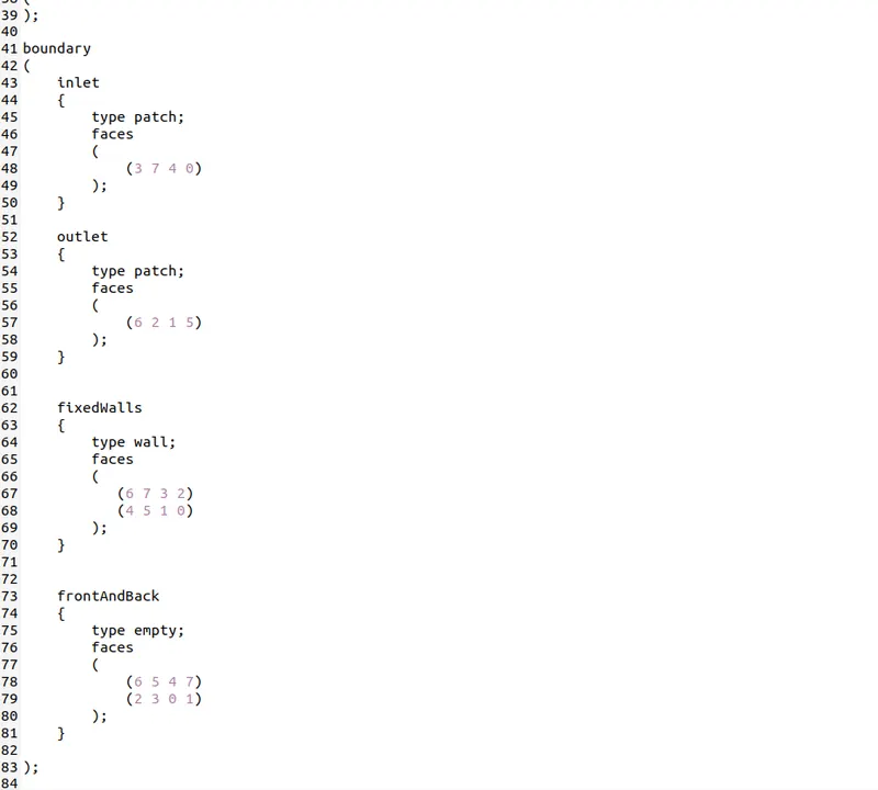
Further in "blockMeshDict" we have to define the boundaries Inlet , Outlet and Fixed walls, we define Inlet and Oulet as a patch since there we need to specify the value of variables and Fixed wall is of the type wall which has a no-slip boundary condition, frontAndBack are specified since we are simulating a 2-D flow field, so hence we do not specify any conditions for the front and Back faces of the Geometry, so they are empty
here we define the appropriate faces from the Geometry
and this is how we create or desired geometry, further we run the command "blockMesh" and this is how Mesh is created, You can also check for the Mesh
This is how the mesh for the above "blockMeshDict" is
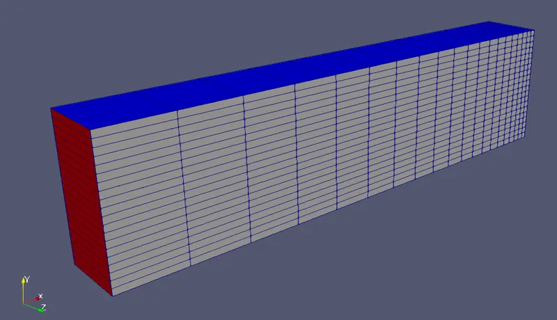
In the Same way we can create the mesh for our original Geometry
The "blockMeshDict" for the Geometry is given as
/*--------------------------------*- C++ -*----------------------------------*\
  =========                 |
  \\      /  F ield         | OpenFOAM: The Open Source CFD Toolbox
   \\    /   O peration     | Website:  https://openfoam.org
    \\  /    A nd           | Version:  9
     \\/     M anipulation  |
\*---------------------------------------------------------------------------*/
FoamFile
{
    format      ascii;
    class       dictionary;
    object      blockMeshDict;
}
// * * * * * * * * * * * * * * * * * * * * * * * * * * * * * * * * * * * * * //

convertToMeters 0.001;

vertices
(
    (0 0 0)
    (80 0 0)
    (80 5 0)
    (0 5 0)
    (0 0 10)
    (80 0 10)
    (80 5 10)
    (0 5 10)
    (0 10 0)
    (80 10 0)
    (0 10 10)
    (80 10 10)
    (80 -10 0)
    (200 -10 0)
    (200 0 0)
    (200 5 0)
    (200 10 0)
    (80 -10 10)
    (200 -10 10)
    (200 0 10)
    (200 5 10)
    (200 10 10)
);

blocks
(
    hex (0 1 2 3 4 5 6 7) (80 5 1) simpleGrading (1 1 1)
    hex (3 2 9 8 7 6 11 10) (80 5 1) simpleGrading (1 1 1)
    hex (1 14 15 2 5 19 20 6) (120 5 1) simpleGrading (1 1 1)
    hex (2 15 16 9 6 20 21 11) (120 5 1) simpleGrading (1 1 1)
    hex (12 13 14 1 17 18 19 5) (120 10 1) simpleGrading (1 1 1)

);

edges
(
);

boundary
(
    inlet
    {
        type patch;
        faces
        (
            (0 3 7 4)
            (3 8 10 7)
        );
    }

    outlet
    {
        type patch;
        faces
        (
            (14 13 18 19)
            (15 14 19 20)
            (16 15 20 21)
        );
    }

    fixedWalls
    {
        type wall;
        faces
        (
            (11 10 8 9)
            (4 5 1 0)
            (9 16 21 11)
            (12 17 18 13)
            (5 17 12 1)
        );
    }
    frontAndBack
    {
        type empty;
        faces
        (
            (0 1 2 3)
            (3 2 9 8)
            (1 14 15 2)
            (2 15 16 9)
            (12 13 14 1)
            (6 5 4 7)
            (11 6 7 10)
            (20 19 5 6)
            (21 20 6 11)
            (19 18 17 5)
        );
    }
);

mergePatchPairs
(

);

// ************************************************************************* //
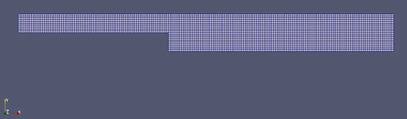
After this we execute the command "blockMesh" and View the Results in ParaView
Step 5:
In this Step we update the Initial conditions Required for the solution
The initial conditions can be specified by going into folder "0" in the case file
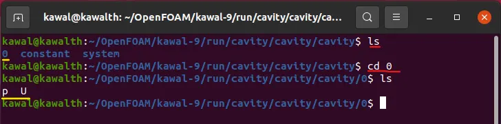
Now we can see two seperate files "p" which is to specify Pressure and "U" to specify Velocity, and since we are solving incompressible-laminar-viscous flow we have only 2 variables "Pressure" and "Velocity" , we solve only Continuity and Momentum Equations
Updating Pressure p : open the file with command "gedit p" and update it
/*--------------------------------*- C++ -*----------------------------------*\
  =========                 |
  \\      /  F ield         | OpenFOAM: The Open Source CFD Toolbox
   \\    /   O peration     | Website:  https://openfoam.org
    \\  /    A nd           | Version:  9
     \\/     M anipulation  |
\*---------------------------------------------------------------------------*/
FoamFile
{
    format      ascii;
    class       volScalarField;
    object      p;
}
// * * * * * * * * * * * * * * * * * * * * * * * * * * * * * * * * * * * * * //

dimensions      [0 2 -2 0 0 0 0];

internalField   uniform 0;

boundaryField
{
    inlet
    {
        type            zeroGradient;
    }

    outlet
    {
	type             fixedValue;
	value            uniform 0;
    }

    fixedWalls
    {
        type            zeroGradient;
    }

    frontAndBack
    {
        type            empty;
    }
}

// ************************************************************************* //
Updating Velocity U , we take the inlet Velocity as U = 1
/*--------------------------------*- C++ -*----------------------------------*\
  =========                 |
  \\      /  F ield         | OpenFOAM: The Open Source CFD Toolbox
   \\    /   O peration     | Website:  https://openfoam.org
    \\  /    A nd           | Version:  9
     \\/     M anipulation  |
\*---------------------------------------------------------------------------*/
FoamFile
{
    format      ascii;
    class       volVectorField;
    object      U;
}
// * * * * * * * * * * * * * * * * * * * * * * * * * * * * * * * * * * * * * //

dimensions      [0 1 -1 0 0 0 0];

internalField   uniform (0 0 0);

boundaryField
{
    inlet
    {
        type            fixedValue;
        value           uniform (1 0 0);
    }

    outlet
    {
	type            zeroGradient;
    }


    fixedWalls
    {
        type            noSlip;
    }

    frontAndBack
    {
        type            empty;
    }
}

// ************************************************************************* //
We also need to update the "controlDict" this file contains important information related to the value of time-step, the start time, the end time and the Writing Interval
/*--------------------------------*- C++ -*----------------------------------*\
  =========                 |
  \\      /  F ield         | OpenFOAM: The Open Source CFD Toolbox
   \\    /   O peration     | Website:  https://openfoam.org
    \\  /    A nd           | Version:  9
     \\/     M anipulation  |
\*---------------------------------------------------------------------------*/
FoamFile
{
    format      ascii;
    class       dictionary;
    location    "system";
    object      controlDict;
}
// * * * * * * * * * * * * * * * * * * * * * * * * * * * * * * * * * * * * * //

application     icoFoam;

startFrom       startTime;

startTime       0;

stopAt          endTime;

endTime         0.1;

deltaT          0.000001;

writeControl    timeStep;

writeInterval   100;

purgeWrite      0;

writeFormat     ascii;

writePrecision  6;

writeCompression off;

timeFormat      general;

timePrecision   6;

runTimeModifiable true;


// ************************************************************************* //
Since this Method is an Explicit Method we have to be careful about the time step size since we have a finer grid we have to take a very small time step to compensate for the finer grid size
Step 6:
Finally After setting up all the necessary condition we need to run the simulation with the solver we have selected that is "icoFoam"
But First we need to execute ./Allclean command to remove all the previously done solution
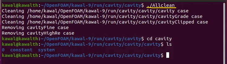
Now we Firstly have to construct mesh, since we cleaned all the previous results
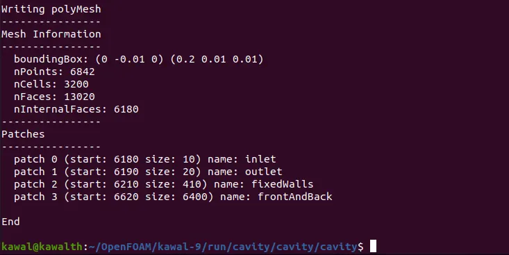
This indicates that the Mesh has been created succesfully, we can also run command "checkMesh" to know the quality of Mesh
Next we run our Iteration by command "icoFoam"

After Executing this command the Calculation will start and depending upon the Processing capability of the Machine the calculation will end after some time
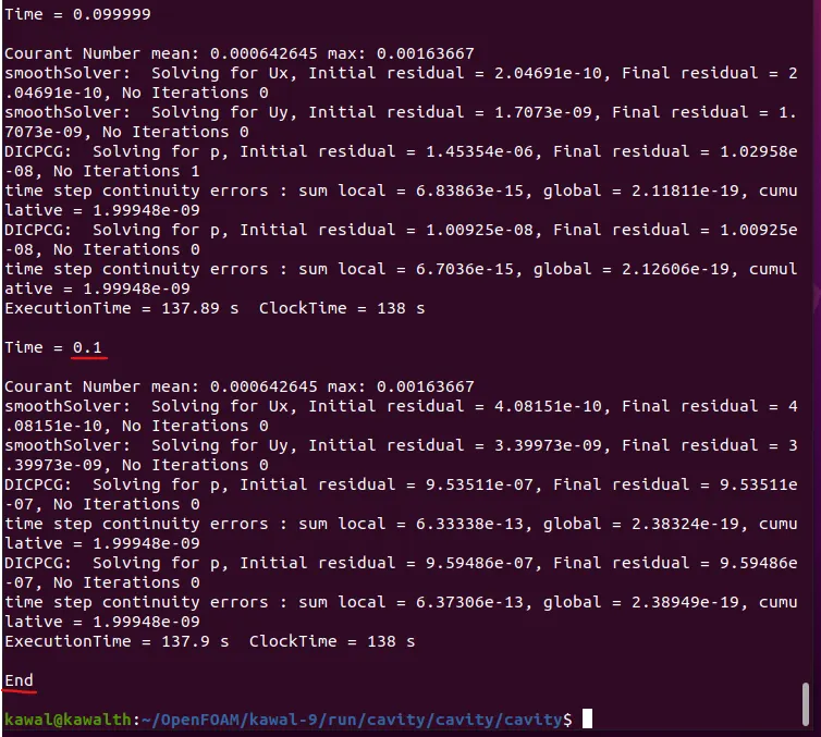
Finally we can Visualize our Results in ParaView by entering the command "paraFoam"

Next a GUI Window will appear as shown below
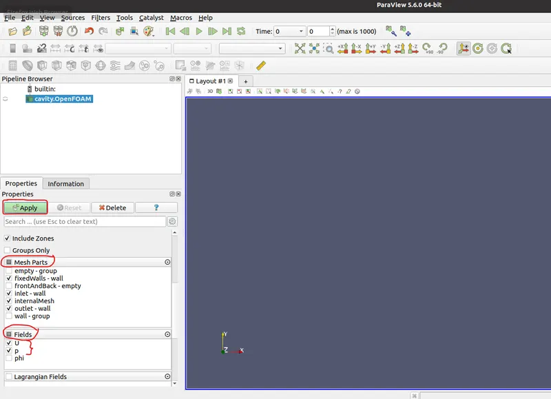
In this window we need to check "Mesh Parts" we tick all the Faces we have describe in the "blockMeshDict" file, further we need to tick the variables we want to visualise in the Fluid Domain, which in our case are Velocity(U) and Pressure(p)
Then we click Apply
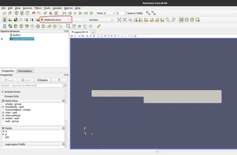
Now we select the required Variable from the drop down menu encircled in red , and we can select to run the simulation with the play button at the upper right portion of the menu.
After Running the Simulation we get the Following Results
CASE 1:
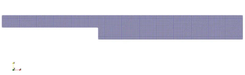
Mesh:
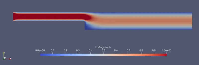
This is the Steady State Velocity in the Fluid Domain at time = 0.2 sec :
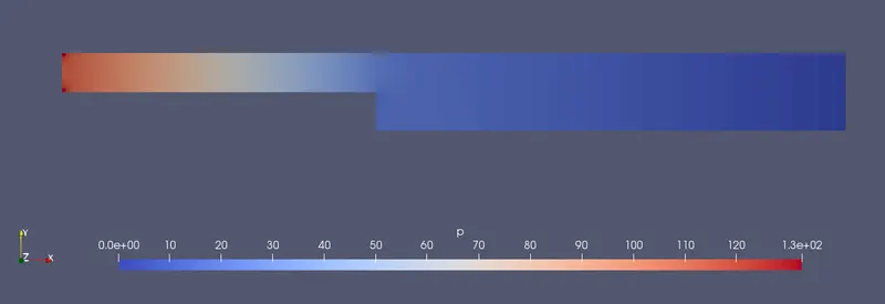
This is the Variation of Pressure in the Fluid Domain :
Output For Case 1 are
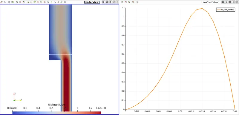
The velocity profile at 0.085 m from the inlet of the geometry for Case 1: (No Grading Factor)
CASE 2:
Now for CASE 2 we have to use the Grading Factor to create a finer Mesh near the walls, and also near the step:
Now for Applying a GF = 0.2 near the walls we need to update the "blocks" section from the "blockMeshDict" and generate the mesh
blocks
(
hex (0 1 2 3 4 5 6 7) (80 5 1) simpleGrading (0.2 5 1)
hex (3 2 9 8 7 6 11 10) (80 5 1) simpleGrading (0.2 0.2 1)
hex (1 14 15 2 5 19 20 6) (120 5 1) simpleGrading (5 5 1)
hex (2 15 16 9 6 20 21 11) (120 5 1) simpleGrading (5 0.2 1)
hex (12 13 14 1 17 18 19 5) (120 10 1) simpleGrading (5 5 1)
);
By making the following change in "blockMeshDict" and running the command "blockMesh" we get the following Mesh
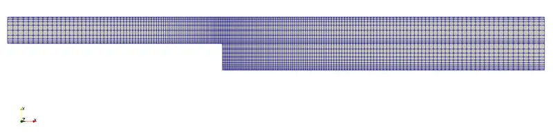
We have now successfully created a finer mesh near the walls and some other critical areas
We further run the calculation for this Mesh file and plot the Velocity and Pressure Profiles
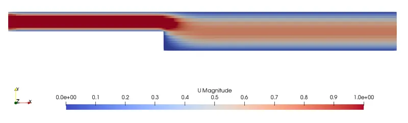
Steady State Velocity Profile in the Fluid Domain at time = 0.2 sec :
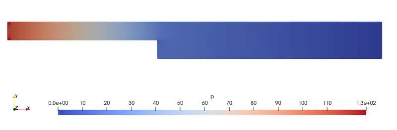
Steady State Variation of Pressure in the Fluid Domain :
Output for CASE 2:
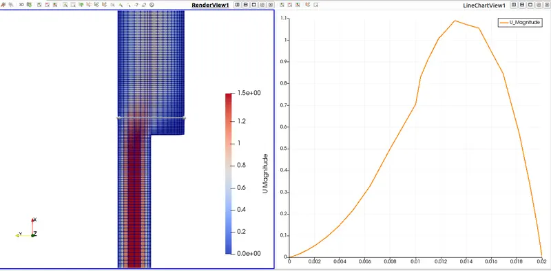
The velocity profile at 0.085 m from the inlet of the geometry for Case 2: (GF = 0.2)
Conclusion:
It can be seen that the profile in CASE 2 retaines it's accuracy near the walls where Velocity changes more abruptly but since we have a slight coarse mesh at the center therefore we get velocities seperated by a larger distance as compared to the profile in CASE 1 which would than affect the accuracy while calculation but since for this part of the profile(center) the change in the velocity is not much abrupt it still manages to retain its accuracy.
If we want to have a more precise computation with minimum resource utilisation(which in this case is time and computational resources) we have to use our understanding of Fluid Physics to guess the area in the Domain where the Flow-Field variables changes abruptely and add a finer Mesh at that section
We have done the same thing in Case 2 where in we obtained much accurate results at the portion of Fluid Domain where the Velocity changes rapidly (which is the important thing while performing any Analysis).
Therefore we conclude that we can obtain more accurate results with a Strategically Graded Mesh