Week 7 - Simulation of a 1D Super-sonic nozzle flow simulation using Macormack Method
AIM:
To analyse a Quasi 1-D flow through a subsonic Convergent Divergent Nozzle using the Conservative and Non-Conservative form of the Governing Equations and Solving them using the MacCormack Method.
ASSUMPTIONS:
- The Flow is Isentropic Flow along X direction.
- The effects due to gravitational Force and Viscous Force are neglected.
- The Fluid behaves as an Ideal Gas.
OBJECTIVES:
- To plot and analyse Steady-state distribution of primitive variables inside the nozzle, these includes Pressure(P), Velocity(V), Temperature(T) and Density(`rho`)
- To plot and analyse Time-wise variation of the primitive variables, for eg. variation of Velocity(V) with time at the throat of the Nozzle.
- To plot and Analyse Variation of Mass flow rate distribution inside the nozzle at different time steps during the time-marching process.
- To plot the Comparison of Normalized mass flow rate distributions of both forms Conservative and Non Conservative Form.
- To Perform a grid independence test on the solution.
- To compare the 2 different forms of the Governing Equations Conservative and Non-Conservative Form and to draw Inferences.
Formulating the Governing Equations:
Now its important to know that there are two forms for Governing Equations for these flow problem Conservative Form and the Non Conservative Form. These both Forms are the same, it follows the same Laws, but are Mathematically Manipulated to suit for our Numerical approach, but it broad terms they are one and the same.
The Analytic Solution for the Steady state Quasi 1-D flow exist, but we still insist on formulating a Numerical Scheme to solve it Numerical to understand it's Unsteady State behaviour and to finally compare our numerical solution with the Analytic Solution to draw our Inferences.
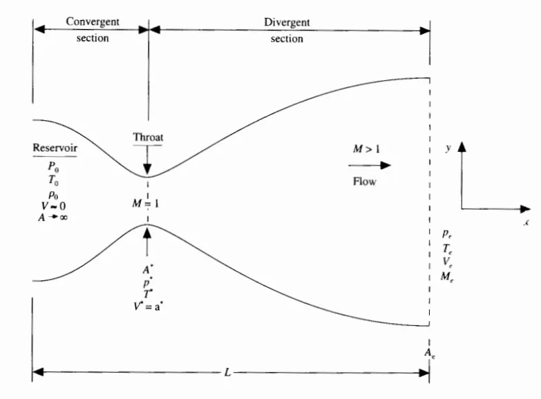
The Nozzle Diagram with Section is given as:
The Nozzle can be split into two sections Convergent and Divergent Section and in between these section lies the throat.
Now we consider a small Section of the Nozzle along x axis with a width of "dx" and we than apply RTT(Reynolds Transport Theorem) to the Control Volume for Mass, Momentum and Energy and this is how we get our Continuity, Momentum and Energy Equations
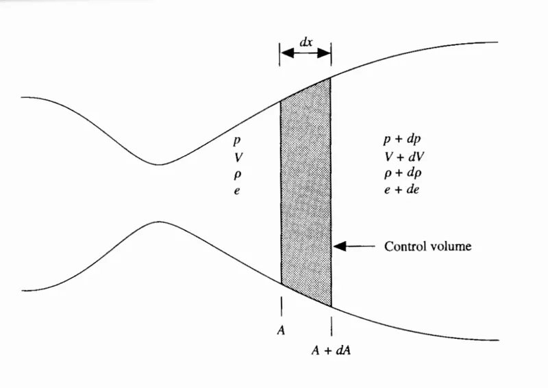
The RTT(Reynolds Transport Theorem) for a CV is given as:
`(delB_"sys")/(delt) = (del)/(dt)intintint_"CV"rhob*dbigvee+intint_"CS" rhob(barV.bardS)`----(I)
here B = any Extensive Property
and b = Intensive version of B ( i.e b = B/mass)
Putting B = Mass , therefor b = 1 we get
`(delM_"sys")/(delt) = (del)/(delt)intintint_"CV"rho.dbigvee+intint_"CS"rhobarV.bar(dS)`----(A)
here `bigvee = "Volume"`
Mass of the system doesn't change with time it remains constant, therefore
`(delM_"sys")/(delt) = 0`----(1.1)
`(del)/(delt)intintint_"CV"rho.dbigvee = (del)/(delt)(rhoA.dx)`-----(1.2)
`intint_"CS"rhobarV.bar(dS) = (rho+drho)(V+dV)(A+dA)-rhoVA`
`intint_"CS"rhobarV.bar(dS) = d(rhoAV)`-----(1.3)
Finally we put Equations (1.1)(1.2)(1.3) into Equation (A) to get
`(del)/(delt)(rhoA) + (del)/(delx)(rhoAV) = 0`
This Equation is the Conservative form of the Continuity Equation
Similarily we can also derive the conservative form of the Momentum Equation using the RTT and by putting
B = M.V and b = V
The Equation (I) will become
`(del(MV)_"sys")/(delt) = (del)/(delt)intintint_"CV"rho.V.dbigvee + intint_"CS" rhoV(barV.bar(dS))`------(B)
`(del(MV)_"sys")/(delt) = -intint_"CS"p.dA`------(2.1)
Since the Rate of change of momentum is the External Force acting along X-axis (with reference to Nozzle), The Force acting for the control surface is given as in Equation (2.2) here its negative sign since the normal from the CS always points outwards and we want the Force to be positive along Positive X-Axis, hence we add a -ve sign to compensate.
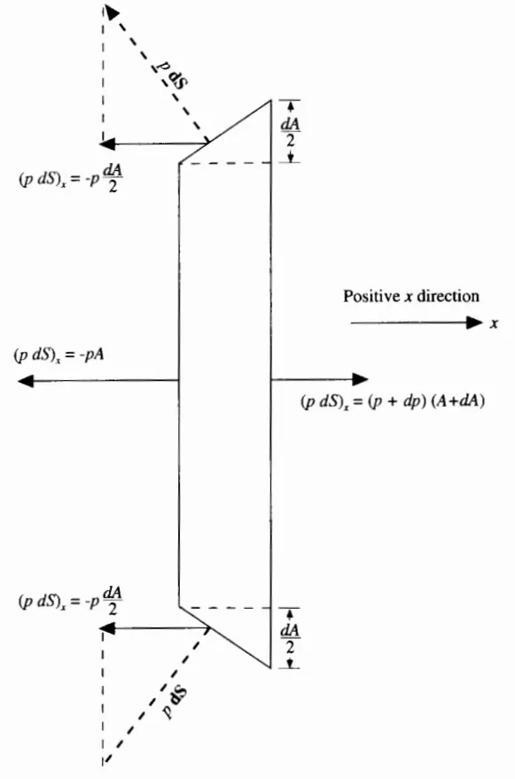
Equation (2.1) can be further solved as
`(del(MV)_"sys")/(delt) = -intint_"CS"p.dA = -{-pA-pdA/2-pdA/2+(p+dp)(A+dA)}`
`(del(MV)_"sys")/(delt) = -intint_"CS"p.dA = -Adp` ------(2.1)
`(del)/(delt)intintint_"CV"rho.V.dbigvee=(del)/(delt)(rhoVA.dx)`-----(2.2)
`intint_"CS" rhoV(barV.bar(dS)) = (rho+drho)(V+dV)^2(A+dA)-rhoV^2A`
`intint_"CS" rhoV(barV.bar(dS)) = d(rhoAV^2)`-------(2.3)
Putting Equations (2.1)(2.2) and (2.3) in Equation (B) we get
`(del)/(delt)(rhoVA.dx)+d(rhoAV^2)=-A.dp`
Further Dividing this Equation by "dx" we get
`(del)/(delt)(rhoVA)+(del(rhoAV^2))/(delx)=-A.(delp)/(delx)`
This is the Conservative form of the Momentum Equation
Now we derive the conservative Form of the Energy Equation with the RTT
Here we consider `B = M(e+V^2/2)` and `b = (e+V^2/2)`
We also have to consider the Kinetic Energy since the fluids are at high velocity, so it cannot be neglected.
`(delE_"sys")/(dt) = (del)/(delt)intintint_"CV"rho(e+V^2/2).dvee+intint_"CS"rho(e+V^2/2).barV.bar(dS)`------(C)
By applying similiar concept as applied for change in Momentum of a system, the energy change in a system is due to the flow energy associated with the fluid since the heat is considered to be zero(isentropic Flow), the heat generated by the viscous effects is Zero since we have neglected the viscous effects, the Energy change in a system can be written as follows,
`(delE_"sys")/(delt) = -intint_"CS"p.barV.bar(ds)`
This can be further written as
`-intint_"CS"p.barV.bar(ds)=-{-pVA+(p+dp)(V+dV)(A+dA)-2(pV(dA)/2)}`-------(3.1)
Further
`(del)/(delt)intintint_"CV"rho(e+V^2/2).dvee =(del(rho(e+V^2/2)Adx))/(dt)`-------(3.2)
`intint_"CS"rho(e+V^2/2).barV.bar(dS) = (rho+drho)(e+de+(V+dV)^2)(V+dV)(A+dA)`------(3.3)
and Further Simplyfying Equations (3.1) (3.2) (3.3) we get
`(del[rho(e+V^2/2)Adx])/(delt)+d[rho(e+V^2/2)VA]=-d(pAV)`
Dividing this Equation by "dx" we get
`(del[rho(e+V^2/2)A])/(delt)+(del[rho(e+V^2/2)VA])/(delx)=-(del(pAV))/(delx)`
This is the Conservative form of Energy Equation
So Therefore the Conservative Form of Continity, Momentum and Energy Equation are as follows
`(del)/(delt)(rhoA) + (del)/(delx)(rhoAV) = 0`-----------------(AA)
`(del)/(delt)(rhoVA)+(del(rhoAV^2))/(delx)=-A.(delp)/(delx)`-------------(BB)
`(del[rho(e+V^2/2)A])/(delt)+(del[rho(e+V^2/2)VA])/(delx)=-(del(pAV))/(delx)`---------(CC)
From these Conservative Form we can derive the Non-Conservative form of the Governing Equations
The Non Conservative Form for the Continuity Equation is the same as the Conservative form.
`(del)/(delt)(rhoA) + (del)/(delx)(rhoAV) = 0`-----(A')
The Non-Conservative Form for the Momentum Equation is obtained by Multiplying Equation (AA) with "V" and then Subtracting it from Equation (BB)
`rhoA(delV)/(delt)+rhoAV(delV)/(delx)=-A(delp)/(delx)`----(B')
The Non Conservative Form of Energy Equation is given by
1. Multiply Equation (BB) with "V" and Subtract it from Equation (CC) to obtain
`(del(rhoeA))/(delt)+(del(rhoeVA))/(delx)=-p(del(AV))/(delx)` --------------(CC')
2. Multiply Equation (AA) with "e", Subtract it from Equation (CC') and than divide the Equation by "A" to obtain the final Result
`rho(dele)/(delt)+rhoV(dele)/(delx)=-p(delV)/(delx)-pV(del(lnA))/(delx)`---------(C')
Organising All the Conservative and Non-Conservative Forms of the Governing Equations for Discretization by Macormack's Method
1.Conservative Form
`(del)/(delt)(rhoA) + (del)/(delx)(rhoAV) = 0`-----------------(AA)
`(del)/(delt)(rhoVA)+(del(rhoAV^2))/(delx)=-A.(delp)/(delx)`-------------(BB)
`(del[rho(e+V^2/2)A])/(delt)+(del[rho(e+V^2/2)VA])/(delx)=-(del(pAV))/(delx)`---------(CC)
2. Non Conservative Form
`(del)/(delt)(rhoA) + (del)/(delx)(rhoAV) = 0`-----(A')
`rhoA(delV)/(delt)+rhoAV(delV)/(delx)=-A(delp)/(delx)`----(B')
`rho(dele)/(delt)+rhoV(dele)/(delx)=-p(delV)/(delx)-pV(del(lnA))/(delx)`---------(C')
It is important to note that it is easy to analyse the non-dimensional version of the above Equations.
Conservative Form
Continuity Equation: `(del(rho'A'))/(delt')+(del(rho'A'V'))/(delx')=0`
Momentum Equation: `(del(rho'A'V'))/(delt')+(del(rho'A'V'^2+1/gammap'A'))/(delx')=1/gammap'(delA')/(delx')`
Energy Equation: `(del[rho'((T')/(gamma-1)+gamma/2V'^2)A'])/(delt')+(del[rho'((T')/(gamma-1)+gamma/2V'^2)V'A'+p'A'V'])/(delx')=0`
Non Conservative Form:
Continuity Equation: `(delrho')/(delt')=rho'(delV')/(delx')-rho'V'(del(lnA'))/(delx')-V'(delp')/(delx')`
Momentum Equation: `(delV')/(delt')=-V'(delV')/(delx')-1/gamma((delT')/(delx')+(T')/(rho')(delrho')/(delx'))`
Energy Equation: `(delT')/(delt')=-V'(delT')/(delx')-(gamma-1)T'[(delV')/(delx')+V'(del(lnA'))/(delx')]`
The Non Dimensional Quantities are
Temperature: `T'=T/T_0`
Density: `rho'=rho/rho_0`
Non Dimensional Distance: `x'=x/L`
Non- Dimensional Velocity: `V' = V/a_0`
where `a_0 = sqrt(gammaRT_0)` is local sonic velocity
Non-Dimensional time: `t' = t/(L/a_0)`
where `L/a_0` is the charactersitics time scale
Non-Dimensional Area: `A' = A/(A"*")`
Note: To make writing Equations easy we will consider replacing the Non-Dimensional variables A' with A, T' with T and so on, though they are replaced with the original one they are still in their Non-Dimensional Form.
Discretization and Solving Non-Dimensional form of Governing Equations by Maccormack Method:
The Mac-cormack method is solved for a Flow-field Variable which can be Velocity, Density or Temperature, if we consider f(x) as our flow field variable, then Mac-cormack method can be solved using the following steps
1. Initial Conditions
Since the Governing Equations are Time marching Equations, they require Initial conditions to further iterate for the time steps, thus we require Initial values of the flow field variable or the values at intial time step
2.Predictor Step
`((delf)/(delt))_p = (f_(i+1)-f_i)/(Deltax)`
The predictor step is calculated using the first order Forward Difference approximation, this approximated time derivative is further used to calculate the solution update in the next step.
3. Solution Update
`f_p = f_"Initial"+((delf)/(delt))_p *Deltat`
where
`f_p` = Flow field variable calulated after the predictor step
`f_"Initial"` = Flow Field variable in the Initial Step
`Deltat` = Time Step Size
4. Corrector Step
`((delf)/(delt))_c = (f_i-f_(i-1))/(Deltax)`
`((delf)/(delt))_"avg" = 0.5(((delf)/(delt))_p +((delf)/(delt))_c)`
5. Final Solution Update
`f_"sol" = f_"Initial" + ((delf)/(delt))_"avg"*Deltat`
`f_"sol"` is the Final Solution of the Flow Field variable for the first time step
For calculating the Final Solution for the next time steps we need to repeat the steps 2,3,4 and 5 for the next time steps.
The MATLAB Code is as follows:
close all
clear
clc

% Number of grid points
n = 31;

% Non Dimensional Number x since L = 1
x = linspace(0,3,n)';
dx = x(3)-x(2);

% Defining number of time steps
nt = 1000;

% Defining the gas Constants
gamma = 1.4;

 %%%%%%%%%%%%%%%%%%%%%% NON-CONSERVATIVE FORM %%%%%%%%%%%%%%%%%%%%%%

% Initial profiles of the variables for the Nozzle
% at time step 1

density     = (1-0.3146*x);                         % Density (kg/m^3)
temperature = (1-0.2314*x);                         % Temperature (K)
velocity    = (0.1+1.09*x).*(temperature.^(1/2));   % Velocity (m/s^2)
area        = 1+2.2*(x-1.5).^2;                     % Area (m^2)

% Finding the index for throat
throat = find(area==min(area));

INT1 = [density temperature velocity area];

SOL1 = non_conservative(x,dx,n,nt,gamma,INT1);

rho_nc = SOL1(:,:,1);                        % Density
V_nc   = SOL1(:,:,2);                        % Velocity
T_nc   = SOL1(:,:,3);                        % Temperature
P_nc   = rho_nc.*T_nc;                       % Pressure
M_nc   = V_nc./sqrt(T_nc);                   % Mach Number
mf_nc  = rho_nc.*(area*ones(1,1000)).*V_nc;  % mass flow rate

%%%%%%%%%%%%%%%%%%%%%%%%% PLOTTING THE RESULTS %%%%%%%%%%%%%%%%%%%%%%%%%

% Variation of primitive variables with time at the throat section
figure(1);
subplot(4,1,1);
plot((1:nt),rho_nc(throat,:),'r','Linewidth',1.2);
xlabel('Time Step','Interpreter','Latex','FontSize',10);
ylabel('Density','Interpreter','Latex','FontSize',10);
grid minor

subplot(4,1,2);
plot((1:nt),P_nc(throat,:),'b','Linewidth',1.2);
xlabel('Time Step','Interpreter','Latex','FontSize',10);
ylabel('Pressure','Interpreter','Latex','FontSize',10);
grid minor

subplot(4,1,3);
plot((1:nt),T_nc(throat,:),'k','Linewidth',1.2);
xlabel('Time Step','Interpreter','Latex','FontSize',10);
ylabel('Temperature','Interpreter','Latex','FontSize',10);
grid minor

subplot(4,1,4);
plot((1:nt),M_nc(throat,:),'g','Linewidth',1.2);
xlabel('Time Step','Interpreter','Latex','FontSize',10);
ylabel('Mach No.','Interpreter','Latex','FontSize',10);
grid minor
sgtitle(sprintf('Variation of variables at throat with timestep\n (NON-CONSERVATIVE FORM)'));

figure(2)
% Variation of Mass Flow rate with the time steps
p1 = plot(x,mf_nc(:,50),'r','Linewidth',1.2);
hold on
p2 = plot(x,mf_nc(:,100),'b','Linewidth',1.2);
hold on
p3 = plot(x,mf_nc(:,300),'k','Linewidth',1.2);
hold on
p4 = plot(x,mf_nc(:,800),'g','Linewidth',1.2);
hold on
grid minor
xlabel('L','Interpreter','Latex','FontSize',14);
ylabel('Mass Flow Rate','Interpreter','Latex','FontSize',14);
title(sprintf('Variation Mass flow rate with length at different time-step\n(NON-CONSERVATIVE FORM)'));
legend([p1,p2,p3,p4],'50th','100th','300th','800th');


%%%%%%%%%%%%%%%%%%%%%%%%% CONSERVATIVE FORM %%%%%%%%%%%%%%%%%%%%%%%%%

% Initial profiles of the variables for the Nozzle
% at time step 1

for i = 1:n
    if(x(i)>=0 && x(i)<=0.5)
        density(i)      = 1;
        temperature(i)  = 1;
    elseif(x(i)>=0.5 && x(i)<=1.5)
        density(i)      = 1-0.366*(x(i)-0.5);
        temperature(i)  = 1-0.167*(x(i)-0.5);
    elseif(x(i)>=1.5 && x(i)<=3)
        density(i)      = 0.634 - 0.3879*(x(i)-1.5);
        temperature(i)  = 0.833 - 0.3507*(x(i)-1.5);
    end
end

velocity = 0.59./(density.*area);

INT2 = [density temperature velocity area];

SOL2 = conservative(x,dx,n,nt,gamma,INT2);

rho_c = SOL2(:,:,1);                      % Density
V_c   = SOL2(:,:,2);                      % Velocity
T_c   = SOL2(:,:,3);                      % Temperature
P_c   = rho_c.*T_c;                       % Pressure
M_c   = V_c./sqrt(T_c);                   % Mach Number
mf_c  = rho_c.*(area*ones(1,1000)).*V_c;  % mass flow rate

%%%%%%%%%%%%%%%%%%%%%%%%% PLOTTING THE RESULTS %%%%%%%%%%%%%%%%%%%%%%%%%

% Variation of primitive variables with time at the throat section
figure(3);
subplot(4,1,1);
plot((1:nt),rho_c(throat,:),'r','Linewidth',1.2);
xlabel('Time Step','Interpreter','Latex','FontSize',10);
ylabel('Density','Interpreter','Latex','FontSize',10);
grid minor

subplot(4,1,2);
plot((1:nt),P_c(throat,:),'b','Linewidth',1.2);
xlabel('Time Step','Interpreter','Latex','FontSize',10);
ylabel('Pressure','Interpreter','Latex','FontSize',10);
grid minor

subplot(4,1,3);
plot((1:nt),T_c(throat,:),'k','Linewidth',1.2);
xlabel('Time Step','Interpreter','Latex','FontSize',10);
ylabel('Temperature','Interpreter','Latex','FontSize',10);
grid minor

subplot(4,1,4);
plot((1:nt),M_c(throat,:),'g','Linewidth',1.2);
xlabel('Time Step','Interpreter','Latex','FontSize',10);
ylabel('Mach No.','Interpreter','Latex','FontSize',10);
grid minor
sgtitle(sprintf('Variation of variables at throat with timestep\n (CONSERVATIVE FORM)')...
    );

figure(4);
% Variation of Mass Flow rate with the time steps
p1 = plot(x,mf_c(:,50),'r','Linewidth',1.2);
hold on
p2 = plot(x,mf_c(:,100),'b','Linewidth',1.2);
hold on
p3 = plot(x,mf_c(:,300),'k','Linewidth',1.2);
hold on
p4 = plot(x,mf_c(:,800),'g','Linewidth',1.2);
hold on
grid minor
xlabel('L','Interpreter','Latex','FontSize',14);
ylabel('Mass Flow Rate','Interpreter','Latex','FontSize',14);
title(sprintf('Variation Mass flow rate with length at different time-step\n(CONSERVATIVE FORM)'));
legend([p1,p2,p3,p4],'50th','100th','300th','800th');
hold off


% Comparing the Normalised mass flow rate of the two forms

figure(5)
plot(x,mf_nc(:,end),'b','Linewidth',1.3);
hold on
plot(x,mf_c(:,end),'r','Linewidth',1.3);
xlabel('Length','Interpreter','Latex','FontSize',14);
ylabel('Mass-Flow-Rate','Interpreter','Latex','FontSize',14);
grid minor
legend('Non Conservative Form','Conservative Form');
title(sprintf('Comparing the Normalised mass flow rate \n of Non conservative and Conservative form'));
hold off

% Comparing the Numerical Solution with the Analytical Solution

% Solving Analytical Equation for Mach Number
g = 1.4;
c = (g-1)/(g+1);
k = 2/(g+1);
in = [1 2.5];
u = 1;
for i = 1:n
    a = area(i);
    % Analytical Function for Mach Number
    af = @(m,c,k,a)((c*(m.^2))-((a*m).^(2*c))+k);
    M_a(i) = fzero(@(m)af(m,c,k,a),in(u));
    if(a == 1)
        u = 2;
    end
end

kk = (1+((g-1)/2)*(M_a.^2));
P_a     = kk.^(-g/(g-1));
rho_a   = kk.^(-1/(g-1));
T_a     = kk.^(-1);

figure(6)
subplot(2,2,1);
hold on
plot(x(2:2:end-1),rho_c(2:2:end-1,end),'ro');
plot(x(1:2:end),rho_nc(1:2:end,end),'b*');
plot(x,rho_a,'k');
xlabel('L');
ylabel('Density');
legend('CON','NON-CON','AYT');
grid minor

subplot(2,2,2);
hold on
plot(x(2:2:end-1),P_c(2:2:end-1,end),'ro');
plot(x(1:2:end),P_nc(1:2:end,end),'b*');
plot(x,P_a,'k');
xlabel('L');
ylabel('Pressure');
grid minor

subplot(2,2,3);
hold on
plot(x(2:2:end-1),T_c(2:2:end-1,end),'ro');
plot(x(1:2:end),T_nc(1:2:end,end),'b*');
plot(x,T_a,'k');
xlabel('L');
ylabel('Temperature');
grid minor

subplot(2,2,4);
hold on
plot(x(2:2:end-1),M_c(2:2:end-1,end),'ro');
plot(x(1:2:end),M_nc(1:2:end,end),'b*');
plot(x,M_a,'k');
xlabel('L');
ylabel('Mach-Number');
grid minor
sgtitle(sprintf('Comparing Conservative, Non conservative form\n Solution with the Analytical Solution'));

clear SOL1 SOL2 rho_nc V_nc M_nc T_nc mf_nc P_nc
clear INT1 INT2 rho_c V_c M_c T_c mf_c P_c p1 p2 p3 p4

%%%%%%%%%%%%%%%%%%%%%% GRID INDEPENDENCY TEST %%%%%%%%%%%%%%%%%%%%%%

% For n = 31,61,91
shapes = {'ro','bx','g-'};
colors = {'r','b','g'};
i = 0;
spacing = [2 4 6];

% For Non-Conservative form
for n = [31,61,91]
    i = i + 1;
    x = linspace(0,3,n)';
    dx = x(3)-x(2);

    % Initial conditions for Non Conservative form
    density     = (1-0.3146*x);                         % Density (kg/m^3)
    temperature = (1-0.2314*x);                         % Temperature (K)
    velocity    = (0.1+1.09*x).*(temperature.^(1/2));   % Velocity (m/s^2)
    area        = 1+2.2*(x-1.5).^2;                     % Area (m^2)

    INT1 = [density temperature velocity area];

    SOL1 = non_conservative(x,dx,n,nt,gamma,INT1);

    % Taking the Steady State Solution
    rho = SOL1(:,nt,1);
    V   = SOL1(:,nt,2);
    T   = SOL1(:,nt,3);
    P   = rho.*T;
    M   = V./sqrt(T);
    MFR = SOL1(:,:,1).*SOL1(:,:,2).*(area*ones(1,nt));

    figure(7);
    subplot(2,2,1)
    hold on
    plot(x(1:spacing(i):end),rho(1:spacing(i):end),shapes{i},'Linewidth',1.2);
    xlabel('L');
    ylabel('Density');
    grid minor
    if(i==3)
        legend('n = 31','n = 61','n = 91');
    end

    subplot(2,2,2)
    hold on
    plot(x(1:spacing(i):end),P(1:spacing(i):end),shapes{i},'Linewidth',1.2);
    xlabel('L');
    ylabel('Pressure');
    grid minor
    if(i==3)
        legend('n = 31','n = 61','n = 91');
    end

    subplot(2,2,3)
    hold on
    plot(x(1:spacing(i):end),T(1:spacing(i):end),shapes{i},'Linewidth',1.2);
    xlabel('L');
    ylabel('Temperature');
    grid minor
    if(i==3)
        legend('n = 31','n = 61','n = 91');
    end

    subplot(2,2,4)
    hold on
    plot(x(1:spacing(i):end),M(1:spacing(i):end),shapes{i},'Linewidth',1.2);
    xlabel('L');
    ylabel('Mach Number ');
    grid minor
    if(i==3)
        legend('n = 31','n = 61','n = 91');
    end
    sgtitle(sprintf("GRID-INDEPENDENCY TEST\nNON-CONSERVATIVE"));

    figure(8);
    % Variation of Mass Flow rate at throat with the time step
    plot(1:nt,MFR(throat,:),colors{i},'Linewidth',1.2);
    xlabel('time step');
    ylabel('Mass-Flow-Rate');
    title(sprintf('Variation of mass-flow-rate with time steps \n for Non-Conservative Form'));
    hold on
    grid minor
    if(i==3)
        legend('n = 31','n = 61','n = 91');
    end

end

clear density area velocity temperature
% For Conservative form
i = 0;
for n = [31,61,91]
    i = i + 1;
    x = linspace(0,3,n)';
    dx = x(3)-x(2);
    area        = 1+2.2*(x-1.5).^2;
    for ij = 1:n
    if(x(ij)>=0 && x(ij)<=0.5)
        density(ij)      = 1;
        temperature(ij)  = 1;
    elseif(x(ij)>=0.5 && x(ij)<=1.5)
        density(ij)      = 1-0.366*(x(ij)-0.5);
        temperature(ij)  = 1-0.167*(x(ij)-0.5);
    elseif(x(ij)>=1.5 && x(ij)<=3)
        density(ij)      = 0.634 - 0.3879*(x(ij)-1.5);
        temperature(ij)  = 0.833 - 0.3507*(x(ij)-1.5);
    end
    end

    velocity = 0.59./(density.*area');

    INT2 = [density' temperature' velocity' area];

    SOL2 = conservative(x,dx,n,nt,gamma,INT2);

    % Taking the Steady State Solution
    rho = SOL2(:,nt,1);
    V   = SOL2(:,nt,2);
    T   = SOL2(:,nt,3);
    P   = rho.*T;
    M   = V./sqrt(T);
    MFR = SOL2(:,:,1).*SOL2(:,:,2).*(area*ones(1,nt));

    figure(9);
    subplot(2,2,1)
    hold on
    plot(x(1:spacing(i):end),rho(1:spacing(i):end),shapes{i},'Linewidth',1.2);
    xlabel('L');
    ylabel('Density');
    grid minor
    if(i==3)
        legend('n = 31','n = 61','n = 91');
    end

    subplot(2,2,2)
    hold on
    plot(x(1:spacing(i):end),P(1:spacing(i):end),shapes{i},'Linewidth',1.2);
    xlabel('L');
    ylabel('Pressure');
    grid minor
    if(i==3)
        legend('n = 31','n = 61','n = 91');
    end

    subplot(2,2,3)
    hold on
    plot(x(1:spacing(i):end),T(1:spacing(i):end),shapes{i},'Linewidth',1.2);
    xlabel('L');
    ylabel('Temperature');
    grid minor
    if(i==3)
        legend('n = 31','n = 61','n = 91');
    end

    subplot(2,2,4)
    hold on
    plot(x(1:spacing(i):end),M(1:spacing(i):end),shapes{i},'Linewidth',1.2);
    xlabel('L');
    ylabel('Mach Number ');
    grid minor
    if(i==3)
        legend('n = 31','n = 61','n = 91');
    end

    sgtitle(sprintf("GRID-INDEPENDENCY TEST\nCONSERVATIVE FORM"));

    figure(10);
    % Variation of Mass Flow rate at throat with the time step
    plot(1:nt,MFR(throat,:),colors{i},'Linewidth',1.2);
    xlabel('time step');
    ylabel('Mass-Flow-Rate');
    title(sprintf('Variation of mass-flow-rate with time steps \n for Conservative Form'));
    hold on
    grid minor
    if(i==3)
        legend('n = 31','n = 61','n = 91');
    end

end
The above code uses two functions to solve for the non-conservative and the conservative form of the Governing Equation
For the Non- Conservative Form we take the initial conditions as
`rho = 1-(0.3146)x`
`T = 1-(0.2314)x`
`V=(0.1+1.09x)T^(1/2)`
and we take the Area profile as
`A = 1+2.2(x-1.5)^(2)` for `0<=x<=3`
The Boundary conditions are as follows
`V(1) = 2*V(2) - V(3)`
`V(n) = 2*V(n-1) - V(n-2)`
`rho(n) = 2*rho(n-1) - rho(n-2);`
`T(n) = 2*T(n-1) - T(n-2)`
So the Length of the Nozzle is considered from x = 0 to x = 3
Here since the solution is solved explicitly the stability of the solution is governed by the CFL(Courant–Friedrichs–Lewy) criteria which states that
CFL number < 0.5 for stability and
`dt = (CFL*dx)/(sqrtT+V)`
This time step will retain the stability of the solution
Note:- The above initial and Boundary conditions come from the book "Computational Fluid Dynamics by John D. Anderson, Jr.".
The function for solving the Non- Conservative form using Mac-cormach Method is as follows.
function [SOL] = non_conservative(x,dx,n,nt,gamma,INT)

SOL = zeros(n,nt,3);

% Initial conditions (INT)
rho     = INT(:,1);       % Density (kg/m^3)
T       = INT(:,2);       % Temperature (K)
V       = INT(:,3);       % Velocity (m/s^2)
A       = INT(:,4);       % Area (m^2)

% Defining CFL Number
C = 0.5;        % For a stable solution

time_sec = 0;
%dt = 0.001;

%Time loop
for k = 1:nt
    d = C.*dx./(sqrt(T)+V);
    dt = min(d);
    % Calculating the time step by CFL number
    time_sec = time_sec + dt;

    % Updating the old values of Primitive Variables
    rho_old = rho;
    V_old   = V;
    T_old   = T;


    % Predictor method
    for i = 2:n-1
        % By Forward Differencing
        drhodx  = (rho(i+1)-rho(i))/dx;
        dVdx    = (V(i+1)-V(i))/dx;
        dTdx    = (T(i+1)-T(i))/dx;
        dlogAdx = (log(A(i+1))-log(A(i)))/dx;


        % Continuity Equation
        drhodt_P(i) = -rho(i)*(dVdx)-rho(i)*V(i)*(dlogAdx)...
            -V(i)*(drhodx);

        % Momentum Equation
        dVdt_P(i)   = -V(i)*(dVdx)-(1/gamma)*(dTdx+(T(i)/rho(i))*drhodx);

        % Energy Equation
        dTdt_P(i)   = -V(i)*(dTdx)-(gamma-1)*(T(i))*...
            (dVdx+V(i)*(dlogAdx));

        % Updating the values of the primitive variables
        rho(i)= rho(i) + drhodt_P(i)*dt;
        V(i)  = V(i)   + dVdt_P(i)*dt;
        T(i)  = T(i)   + dTdt_P(i)*dt;

    end
    % Corrector Method
    for i = 2:n-1
        % By Backward Differencing
        drhodx  = (rho(i)-rho(i-1))/dx;
        dVdx    = (V(i)-V(i-1))/dx;
        dTdx    = (T(i)-T(i-1))/dx;
        dlogAdx = (log(A(i))-log(A(i-1)))/dx;


        % Continuity Equation
        drhodt_C(i) = -rho(i)*(dVdx)-rho(i)*V(i)*(dlogAdx)...
            -V(i)*(drhodx);

        % Momentum Equation
        dVdt_C(i)   = -V(i)*(dVdx)-(1/gamma)*(dTdx+(T(i)/rho(i))*drhodx);

        % Energy Equation
        dTdt_C(i)   = -V(i)*(dTdx)-(gamma-1)*(T(i))*...
            (dVdx+V(i)*(dlogAdx));

        % Calculating the average value of time derivative
        % of primitive variables
        drhodt(i) = 0.5*(drhodt_P(i)+drhodt_C(i));
        dVdt(i) = 0.5*(dVdt_P(i)+dVdt_C(i));
        dTdt(i) = 0.5*(dTdt_P(i)+dTdt_C(i));

        % Updating the values of the primitive variables
        % Using the average value
        rho(i)= rho_old(i) + drhodt(i)*dt;
        V(i)  = V_old(i)   + dVdt(i)*dt;
        T(i)  = T_old(i)   + dTdt(i)*dt;

    end

    % Updating the Boundary Conditions
    % Boundary Conditions
    % At Inlet
    %rho(1) = 1;
    %T(1)   = 1;
    V(1)   = 2*V(2) - V(3);
    % At Outlet
    V(n)   = 2*V(n-1) - V(n-2);
    rho(n) = 2*rho(n-1) - rho(n-2);
    T(n)   = 2*T(n-1) - T(n-2);

    % Printing the primitive Variables for Debugging
    fprintf("\n\nTIME-STEP = %g , time = %g sec\n",k,time_sec);
    fprintf("%10s|%10s|%10s|%10s\n",'x','Den(rho)','Vel(V)','Temp(T)');
    fprintf("-------------------------------------------\n");
    for i = 1:n
        fprintf(1,"%10g|%10g|%10g|%10g\n",x(i),rho(i),V(i),T(i));
    end
    fprintf("-------------------------------------------\n");
    SOL(:,k,1) = rho;
    SOL(:,k,2) = V;
    SOL(:,k,3) = T;
end
end
Now for the Conservative form, we cannot solve the conservative form with the primitive variables using Mac-cormack Method, since this will magnify the errors in the primitive variables and will affect the stability of the solution
Hence we introduce a new set of variables and flux which are compatible with the Mac-cormack's Method
`U_1 = rhoA`
`U_2=rhoAV`
`U_3 = rho((e)/(gamma-1)+(gamma)/(2)V^2)A`
`F_1 = rhoAV`
`F_2 = rhoAV^2+1/gammapA`
`F_3 = rho((e)/(gamma-1)+(gamma)/(2)V^2)VA+pAV`
`J_2 = 1/gammap(delA)/(delx)`
By replacing these in the original Equation we get the new Equations as
`(delU_1)/(delt)=-(delF_1)/(delx)`
`(delU_2)/(delt)=-(delF_2)/(delx)+J_2`
`(delU_3)/(delt)=-(delF_3)/(delx)`
We further have to represent the values of `F_1,F_2,F_3` in terms of `U_1,U_2,U_3` since we cannot represent it in the form of primitive variables since it would magnify the error
`F_1 = U_2`
`F_2 = (U_2^2)/(U_1)+(gamma-1)/(gamma)(U_3-gamma/2(U_2^2)/(U_1))`
`F_3 = gamma(U_2U_3)/(U_1)-(gamma(gamma-1))/(2)(U_2^3)/(U_1^2)`
`J_2 =(gamma-1)/(gamma)(U_3-gamma/2(U_2^2)/(U_1))(del(lnA))/(delx)`
We can further extract our primitive variables from `U_1,U_2,U_3` as follows
`V = U_2/U_1`
`rho = U_1/A`
`T = (gamma-1)(U_3/U_1-gamma/2V^2)`
In case of the conservative form the initial conditions are as follows
`{:(,rho = 1,),(,T = 1,):} }0<=x<=0.5`
`{:(,rho=1-0.366(x-0.5),),(,T=1-0.167(x-0.5),):}}0.5<=x<=1.5`
`{:(,rho = 0.634-0.3879(x-1.5),),(,T = 0.833-0.3507(x-1.5),):}}1.5<=x<=3`
`V = 0.59/(rhoA)`
The Boundary Conditions are given for the Modified Variables `U_1,U_2,U_3` and they are
At Inlet we have
`U_1()=rho(1)*A(1)`
`U_2(1)=2*U_2(2)-U_2(3)`
`V(1) = (U_2(1))/(U_1(1))`
`U_3(1) = U_1(1)((T(1))/(gamma-1)+(gamma*V(1)^2)/(2))`
At Oulet we have
`U_1(n) = 2U_1(n-1)-U_1(n-2)`
`U_2(n) = 2U_2(n-1)-U_2(n-2)`
`U_3(n) = 2U_3(n-1)-U_3(n-2)`
Since we solve the Conservative form Explicitly the stability of the solution is governed by the CFL(Courant–Friedrichs–Lewy) criteria which states that for a solution to be stable,
CFL<0.5
`dt = (CFL*dx)/(sqrtT+V)`
the value of "dt" from the above Equation retains the stability of the solution.
The MATLAB code for the following is given as
function [SOL] = conservative(x,dx,n,nt,gamma,INT)

SOL = zeros(n,nt,3);
% Initial conditions (INT)
rho     = INT(:,1);       % Density (kg/m^3)
T       = INT(:,2);       % Temperature (K)
V       = INT(:,3);       % Velocity (m/s^2)
A       = INT(:,4);       % Area (m^2)
%
% figure
% plot(x,rho);
% figure
% plot(x,T);
% figure
% plot(x,V);

% Defining CFL Number
C = 0.5;        % For a stable solution

% Updating the Initial Time step for Solution Variables
% from the primitive variables
U1 = rho.*A;
U2 = rho.*A.*V;
U3 = rho.*A.*((T./(gamma-1))+((V.^2).*(gamma/2)));

time_sec = 0 ;
%dt = 0.001;
% TIME LOOP
for k = 1:nt

    % Calculating the time step by CFL Method
    dt = min(C.*dx./(sqrt(T)+V));
    time_sec = time_sec + dt;

    % Copy of old variables
    U1_old = U1;
    U2_old = U2;
    U3_old = U3;

    % Calulcating the Flus vector
    F1 = U2;
    F2 = ((U2.^2)./U1) + ((gamma-1)./gamma).*...
        (U3-(gamma/2).*((U2.^2)./U1));
    F3 = ((U3.*U2.*gamma)./(U1))-((gamma.*(gamma-1))).*((U2.^3)./(2*U1.^2));

    %SPACE LOOP(Mac-cormacks' Method)
    %Predictor Method
    for i = 2:n-1
        % Updating the Source Term
        J2(i) = (1/gamma)*rho(i)*T(i)*((A(i+1)-A(i))/dx);

        % Applying Forward Difference Method
        % Continuity Equation
        dU1dt_P(i) = -(F1(i+1)-F1(i))/dx;

        % Momentum Equation
        dU2dt_P(i) = -((F2(i+1)-F2(i))/dx) + J2(i);

        % Energy Equation
        dU3dt_P(i) = -(F3(i+1)-F3(i))/dx;

        % Updating the Variable by Predictor step
        U1(i) = U1(i) + dU1dt_P(i)*dt;
        U2(i) = U2(i) + dU2dt_P(i)*dt;
        U3(i) = U3(i) + dU3dt_P(i)*dt;
    end

    % Updating the Flux Variables with updated values of
    % U1,U2,U3
    F1 = U2;
    F2 = ((U2.^2)./U1)+((gamma-1)./gamma).*...
        (U3-(gamma/2).*((U2.^2)./U1));
    F3 = ((U3.*U2.*gamma)./(U1))-((gamma.*(gamma-1))).*((U2.^3)./(2*U1.^2));

    %Corrector Method
    for i = 2:n-1
        % Updating the Source Term
        J2(i) = (1/gamma)*rho(i)*T(i)*((A(i)-A(i-1))/dx);

        % Applying Backward Difference Method
        % Continuity Equation
        dU1dt_C(i) = -(F1(i)-F1(i-1))/dx;

        % Momentum Equation
        dU2dt_C(i) = -((F2(i)-F2(i-1))/dx) + J2(i);

        % Energy Equation
        dU3dt_C(i) = -(F3(i)-F3(i-1))/dx;

        % Updating the Final Solution'
        dU1dt(i) = 0.5*(dU1dt_P(i)+dU1dt_C(i));
        dU2dt(i) = 0.5*(dU2dt_P(i)+dU2dt_C(i));
        dU3dt(i) = 0.5*(dU3dt_P(i)+dU3dt_C(i));

        % Final Solution Update
        U1(i) = U1_old(i) + dU1dt(i)*dt;
        U2(i) = U2_old(i) + dU2dt(i)*dt;
        U3(i) = U3_old(i) + dU3dt(i)*dt;

    end

    % Updating the Boundary Conditions
    % At Inlet
    U1(1) = rho(1)*A(1);
    U2(1) = 2*U2(2)-U2(3);

    V(1)  = U2(1)/U1(1);
    U3(1) = U1(1)*((T(1)/(gamma-1))+(gamma*(V(1)^2)/2));

    % At Outlet
    U1(n) = 2*U1(n-1)-U1(n-2);
    U2(n) = 2*U2(n-1)-U2(n-2);
    U3(n) = 2*U3(n-1)-U3(n-2);

    %Updating the primitive variables
    for c = 1:n
        V(c)   = U2(c)/U1(c);
        rho(c) = U1(c)/A(c);
        T(c)   = (gamma-1)*((U3(c)/U1(c))-(gamma/2)*(V(c)^2));
    end

    % Printing the primitive Variables for Debugging
    fprintf("\n\nTIME-STEP = %g , time = %g sec\n",k,time_sec);
    fprintf("%10s|%10s|%10s|%10s\n",'x','Den(rho)','Vel(V)','Temp(T)');
    fprintf("------------------------------------------------------------------------\n");
    for i = 1:n
        fprintf("%10g|%10g|%10g|%10g\n",x(i),rho(i),V(i),T(i));
    end
    SOL(:,k,1) = rho;
    SOL(:,k,2) = V;
    SOL(:,k,3) = T;
end
end
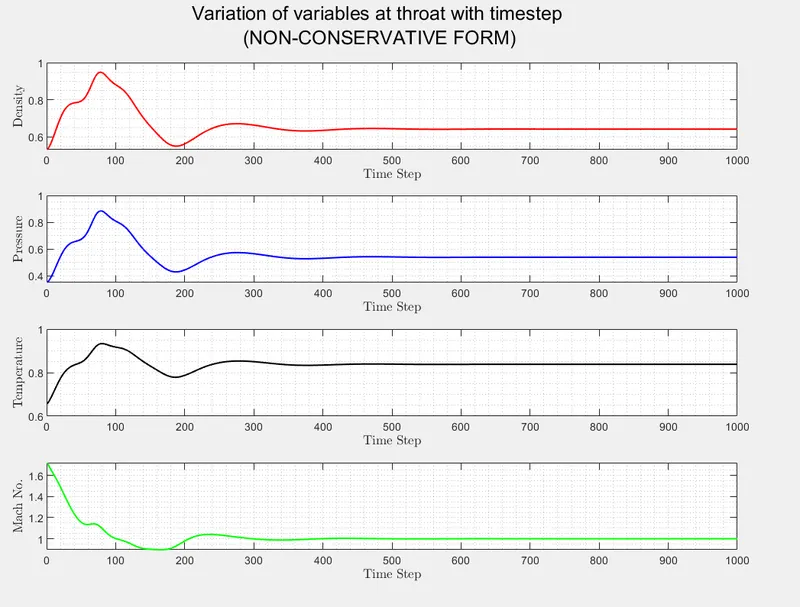
The Results from the above MATLAB code are obtained in the form of plots of the Flow Field Variables
1. Variation of the Flow-Field Variable with the time steps
Non-Conservative Form (FIG-1.1)
Conservative Form(FIG-1.2)
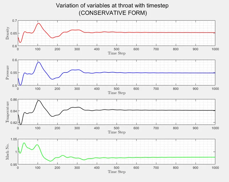
From FIG-1.1 and FIG 1.2 we can visualise the variation of different flow field variables with respect to the time step
It can be concluded that in both the form the variables attain a steady state after 600th-700th time step
2. Variation of Mass-Flow-Rate with time step along the Nozzle Length
Non-Conservative Form (FIG-2.1)
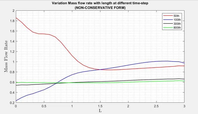
Conservative Form (FIG-2.2)
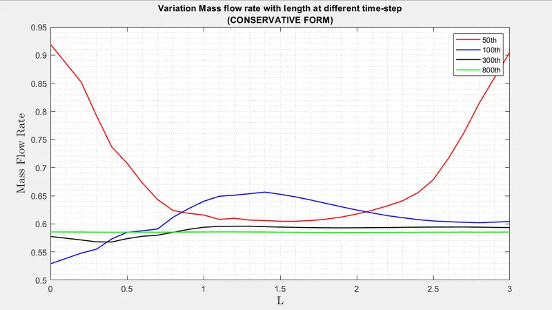
From FIG-2.1 and FIG-2.2 we conclude that the mass-flow-rate is attaining steady-state in both the forms as we proceed in time steps, it can be seen that the difference in the time step 300th and time step 800th is very less compared to that between time step 50th and 100th, it means that the solution is converging.
3. Comparison of Normalised Mass-Flow rate of Conservative and Non-Conservative forms
FIG(3.1)
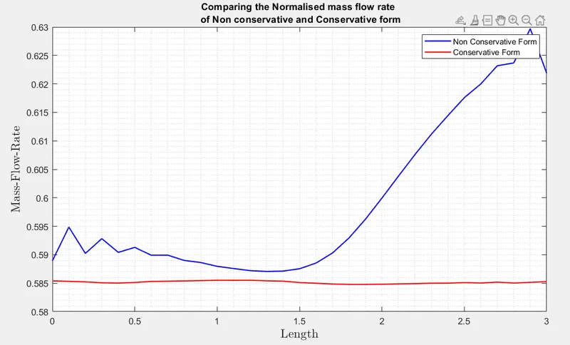
From FIG-3.1 we conclude that as compared to Non-conservative form the conservative form is more stable and has the least variation after attaining the steady state.
4. Comparing the Non-Conservative form, Conservative form with the Analytical Solution
The Analytical Solution for the Steady State distribution of the Flow-Field Variables is given as
`A^2 = 1/M^2[2/(gamma+1)(1+(gamma-1)/1M^2)]^((gamma+1)/(gamma-1))`
`p = [1+(gamma-1)/1M^2]^(-(gamma)/(gamma-1))`
`rho = [1+(gamma-1)/1M^2]^(-(1)/(gamma-1))`
`T = [1+(gamma-1)/1M^2]^-1`
We Solve the Above Equations to Find out the Analytical Solution, we start with finding Mach Number from the Area profile, than proceeding with the other variables.
FIG-4.1
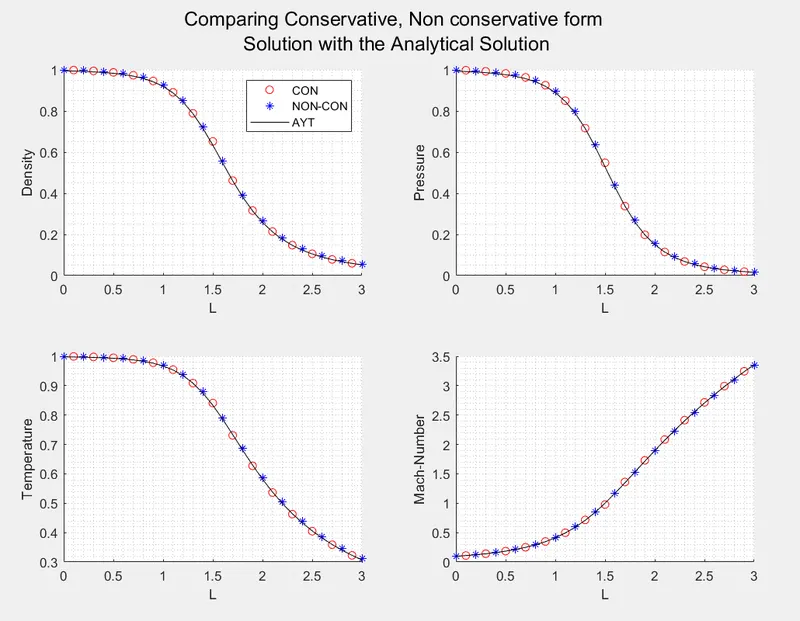
From FIG-4.1 we conclude that the steady state variation of the Flow-Field Variables solved using Conservative and Non-conservative forms of Governing equations fits well when compared to the Analytical Solution with minimum error,
5. Grid Independency Test
Here we consider 3 cases where in 1st case we have 31 grid points, in 2nd Case we have 61 grid points and in 3rd case we have 91 grid points.
We compare the variation of Flow field Variables from the 3 cases and conclude our results
Non-Conservative form (FIG-5.1)
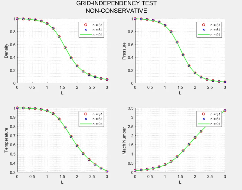
FIG(5.2)
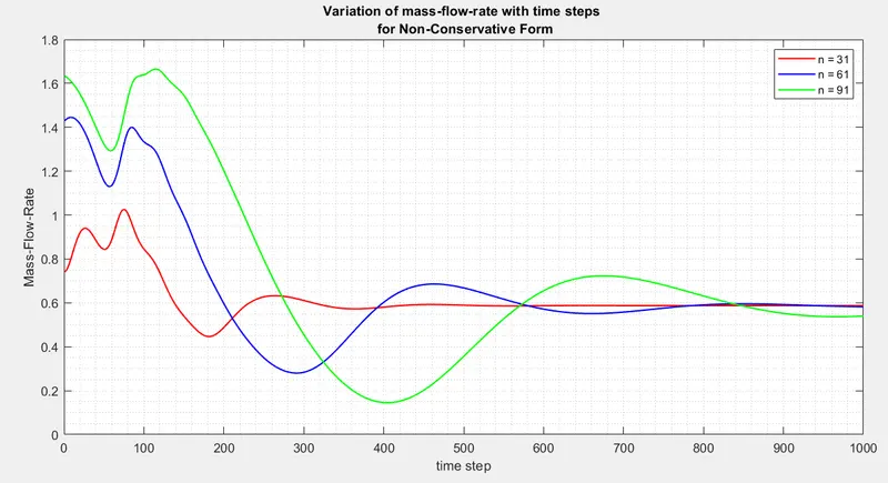
Conservative Form (FIG-5.3)
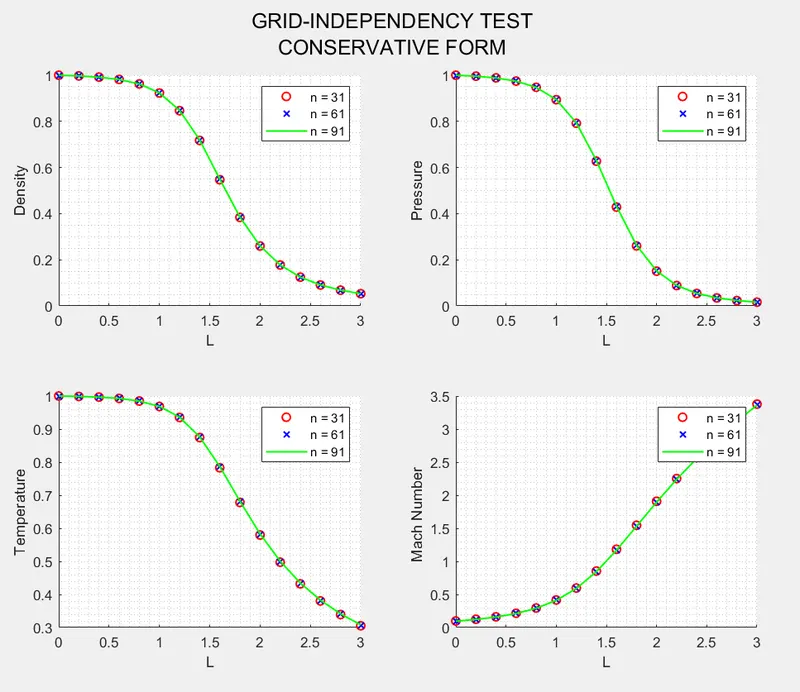
(FIG-5.4)
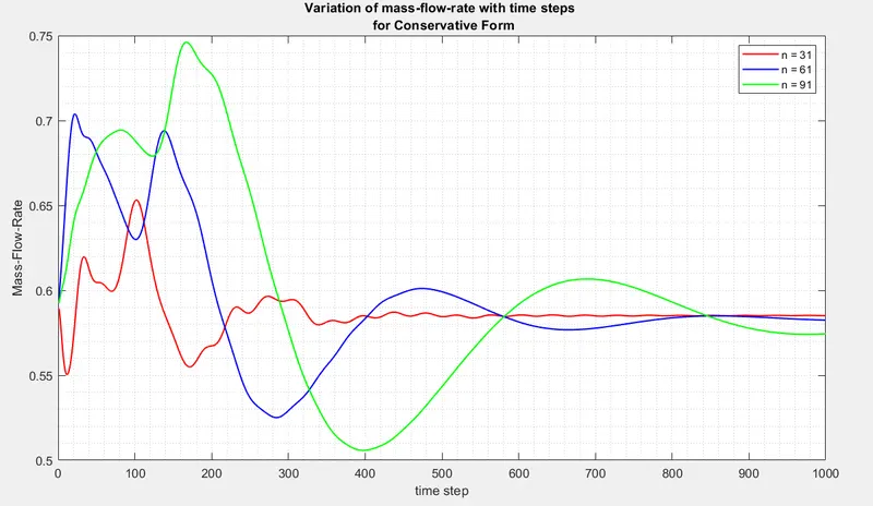
From (FIG-5.1) and (FIG-5.3) we conclude that the Steady-State Solution is independent of Grid although there are variations in (FIG-5.2) and (FIG-5.4), these variations are in the both forms, therefor we conclude that the transient Solution shows variation as we change the grid size hence we conclude that the overall Solution is Grid-Dependent
Conclusion:
From the above results we conclude that the conservative form of the Governing Equations gives consisitent Steady State Results as compared to the Non-Conservative form when we compare the Normalised Mass-Flow rate and also it requires less number of Iterations to attain the Steady State solution.