Week 11 - Simulation of Flow through a pipe in OpenFoam
Problem Statement:
To simulate an axis-symmeteric flow through a pipe by applying wedge boundary conditions, the flow is Laminar and has an inlet Reynolds number as Re = 2100 and we have to validate the steady flow velocity distribution of a fully developed Laminar Flow with the velocity distribution obtained by solving Hagen- Poiseuille's equations which are for a flow through a pipe
Assumptions:
1. The Flow is Steady, incompressible and Laminar.
2. The effects of gravity are negligible only viscous effects are dominant.
3. The velocity along Y-axis is negligible.
In this project we intend to simulate flow through a pipe, the flow will be Laminar with Reynold's No. = 2100. The complete simulation of a cylindrical element would be computationally costly so we consider only a section of this cylinder, a section of say 4 deg. We consider this since the flow is axi-symmetric and we have the same profile on the other side of the axis.
The velocity profile for the Laminar flow through a cylindrical pipe changes from entrance of the pipe until it reaches " Le " which is the Hydrodynamic Entrance Length, Beyond the Hydrodynamic Entrance Region the velocity profile remains unchanged and this is called as Fully Developed Laminar flow.
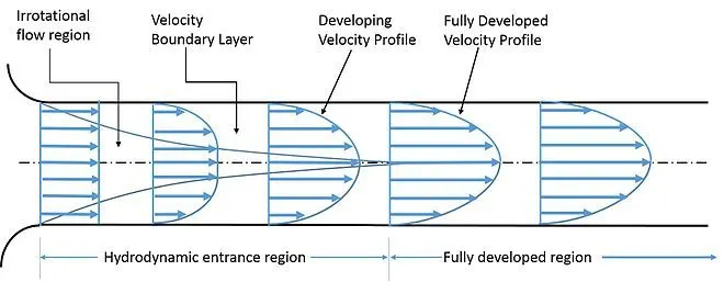
The Figure above shows how the velocity profile changes as the Fluid passes the Hydrodynamic Entrance Region
The velocity profile for the fully developed Laminar Flow can be evaluated using the Hagen-Poiseuille's equations
The Hagen-Poiseuille's equations can be derived from Navier's Stokes Equation applied to a flow along X-axis after which we get
`r(dp)/(dx)=mu(d)/(dr)(r(du)/(dr))`
From which we can derive the velocity profile Equation in terms of 'r' which is the radial distance from the centre of the pipe, we can also evaluate the shear stress distribution along the c/s of the pipe.
The Hydrodynamic Entrance Lenght can be evaluated as
`L_e = 0.06*Re*D`
Where Re = Reynold's Number and D = Diameter(m) of the pipe
`u(r) = R^2/(4mu)((dp)/(dx))[1-(r^2)/(R^2)]`
where `R = D/2`
`V_"avg" = R^2/(4mu)(dp)/(dx)`
`V_"max"= 2V_"avg"` The maximum velocity is at the centre (r = 0)
`(dp)/(dx)=(8muV_"avg")/(R^2)`
`DeltaP = (8muLV"avg")/(R^2)`
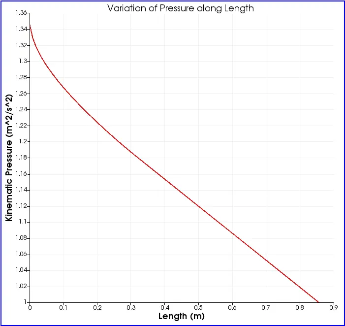
Here important thing to note is that there is a pressure drop at the outlet
The Shear Stress variation can be calculated using Newton's Law of viscocity
`tau = (4muV"avg".r)/(R^2)`
The Maximum shear stress occurs at the walls of the pipe
Now to proceed with we have given the Reynold's Number of the Flow Re = 2100, from this we calculate the average velocity `V_"avg"`
`Re = (rho.V_"avg".D)/(mu)`
From `V_"avg"` we can evaluate the velocity profile and the shear stress profile of a fully developed Laminar Flow by the following Equation
`u(r)=2V_"avg"[1-(r^2)/(R^2)]`
`tau = (4muV"avg".r)/(R^2)`
Here we assume that the Diameter of the pipe is "60 mm"
The viscosity of the Fluid (water) in this case is given at 20deg Celcius Temperature is
`mu = 1.0016" x "10^-3" " (Ns)/m^2`
The Density of water is given as
`rho = 997 " " (kg)/m^3`
Hence the Kinematic Viscosity (`nu`) is given as `nu = mu/rho`
`nu = 1.0046" x "10^(-6) " "(m^2)/s`
For our analysis we consider the Length of the pipe to be slightly greater than the Entrance Length `L_e`
In the Following MATLAB code we consider the wedge to be of 4 deg and we evaluate the vertices of the Fluid Domain and generate the "blockMeshDict" for further generating the blockMesh for the Analysis
We also add Mesh grading at the inlet region since it is the area of abrupt change of velocity
% Solving for Hagen Pousielle's Flow
clc
clear
close all

% Solving for Hagen Pousielle's Flow
% We assume a Reynold's Number of Re = 2100
Re = 2100;
% and Diameter of the Pipe is assume as
D   = 0.006;         % Diameter of Pipe in (m)
mu  = 1.0016e-3;     % Viscosity of Water (Pa.s) at 20 deg Celcius
rho = 997;           % Density of water (kg/m^3) at 20 deg Celcius
L = Re*D*0.06+0.1 ; % Length of the pipe in (m)
R = D/2;             % Radius of pipe

% Calculating the Average Velocity by using Re = (rho.V.D)/(mu)
Vavg = Re*mu/(rho*D);       % Average velocity
Vmax = 2*Vavg;              % Maximum Velocity
DP = 8*mu*L*Vavg/(R^2);     % Pressure Variation
KDP = DP/rho;               % Kinematic Pressure (m^2/s^2)
nu = mu/rho;                % Kinematic Viscosity
% Calculating the Vertices of the fluid Element
theta = 4;      % Angle of wedge in (deg)

x0 = 0;
y0 = 0;
z0 = 0;

x1 = 0;
y1 = R*cosd(theta/2);
z1 = -R*sind(theta/2);

x2 = 0;
y2 = y1;
z2 = -z1;

x3 = L;
y3 = 0;
z3 = 0;

x4 = L;
y4 = y1;
z4 = z1;

x5 = L;
y5 = y2;
z5 = z2;

f1 = fopen('blockMeshDict','w');

% The headers
h1 = '/*--------------------------------*- C++ -*----------------------------------*\';
h2 = '  =========                 |';
h3 = '  \\      /  F ield         | OpenFOAM: The Open Source CFD Toolbox';
h4 = '   \\    /   O peration     | Website:  https://openfoam.org';
h5 = '    \\  /    A nd           | Version:  9';
h6 = '     \\/     M anipulation  |';
h7 = '\*---------------------------------------------------------------------------*/';
h8 = '// * * * * * * * * * * * * * * * * * * * * * * * * * * * * * * * * * * * * * //';

fprintf(f1,'%s\n',h1);
fprintf(f1,'%s\n',h2);
fprintf(f1,'%s\n',h3);
fprintf(f1,'%s\n',h4);
fprintf(f1,'%s\n',h5);
fprintf(f1,'%s\n',h6);
fprintf(f1,'%s\n',h7);

fprintf(f1,'%s\n','FoamFile');
fprintf(f1,'%s\n','{');
fprintf(f1,'\t%s\t%s\n','format','ascii;');
fprintf(f1,'\t%s\t%s\n','class','dictionary;');
fprintf(f1,'\t%s\t%s\n','object','blockMeshDict;');
fprintf(f1,'%s\n','}');
fprintf(f1,'%s\n\n',h8);
fprintf(f1,'%s\n\n','convertToMeters 1;');
fprintf(f1,'%s\n','vertices');
fprintf(f1,'%s\n','(');

fprintf(f1,'\t(%d %d %d)\n',x0,y0,z0);
fprintf(f1,'\t(%d %d %d)\n',x1,y1,z1);
fprintf(f1,'\t(%d %d %d)\n',x2,y2,z2);
fprintf(f1,'\t(%d %d %d)\n',x3,y3,z3);
fprintf(f1,'\t(%d %d %d)\n',x4,y4,z4);
fprintf(f1,'\t(%d %d %d)\n',x5,y5,z5);

fprintf(f1,'%s\n\n',');');

fprintf(f1,'blocks\n');
fprintf(f1,'(\n');
fprintf(f1,'\thex (2 5 3 0 1 4 3 0) (500 50 1) simpleGrading (20 1 1)\n');
fprintf(f1,');\n\n');

fprintf(f1,'edges\n');
fprintf(f1,'(\n');
fprintf(f1,'\tarc 1 2 (%d %d %d)\n',0,R,0);
fprintf(f1,'\tarc 4 5 (%d %d %d)\n',L,R,0);
fprintf(f1,');\n\n');

fprintf(f1,'boundary\n');
fprintf(f1,'(\n');

fprintf(f1,'\tinlet\n');
fprintf(f1,'\t{\n');
fprintf(f1,'\t\ttype patch;\n');
fprintf(f1,'\t\tfaces\n');
fprintf(f1,'\t\t(\n');
fprintf(f1,'\t\t\t(0 1 2 0)\n');
fprintf(f1,'\t\t);\n');
fprintf(f1,'\t}\n\n');

fprintf(f1,'\toutlet\n');
fprintf(f1,'\t{\n');
fprintf(f1,'\t\ttype patch;\n');
fprintf(f1,'\t\tfaces\n');
fprintf(f1,'\t\t(\n');
fprintf(f1,'\t\t\t(3 5 4 3)\n');
fprintf(f1,'\t\t);\n');
fprintf(f1,'\t}\n\n');

fprintf(f1,'\tfixedWall\n');
fprintf(f1,'\t{\n');
fprintf(f1,'\t\ttype wall;\n');
fprintf(f1,'\t\tfaces\n');
fprintf(f1,'\t\t(\n');
fprintf(f1,'\t\t\t(2 1 4 5)\n');
fprintf(f1,'\t\t);\n');
fprintf(f1,'\t}\n\n');

fprintf(f1,'\tfront\n');
fprintf(f1,'\t{\n');
fprintf(f1,'\t\ttype wedge;\n');
fprintf(f1,'\t\tfaces\n');
fprintf(f1,'\t\t(\n');
fprintf(f1,'\t\t\t(1 0 3 4)\n');
fprintf(f1,'\t\t);\n');
fprintf(f1,'\t}\n\n');

fprintf(f1,'\tback\n');
fprintf(f1,'\t{\n');
fprintf(f1,'\t\ttype wedge;\n');
fprintf(f1,'\t\tfaces\n');
fprintf(f1,'\t\t(\n');
fprintf(f1,'\t\t\t(2 5 3 0)\n');
fprintf(f1,'\t\t);\n');
fprintf(f1,'\t}\n\n');

fprintf(f1,'\taxis\n');
fprintf(f1,'\t{\n');
fprintf(f1,'\t\ttype empty;\n');
fprintf(f1,'\t\tfaces\n');
fprintf(f1,'\t\t(\n');
fprintf(f1,'\t\t\t(0 3 3 0 )\n');
fprintf(f1,'\t\t);\n');
fprintf(f1,'\t}\n\n');

fprintf(f1,');\n\n');

fprintf(f1,'mergePatchPairs\n');
fprintf(f1,'(\n');
fprintf(f1,');\n\n');

fprintf(f1,'%s\n',h8);
fclose(f1);

Vavg
nu
KDP
From this we get a "blockMeshDict" file which we copy in our OpenFoam case file and thereafter generate the blockMesh.
We give the initial velocity `V_avg` as our initial condition and we update the value of `nu` in "transportproperties" file
We give the boundary condition for output pressure as the value we obtained from KDP (which is a Kinematic Pressure)
Since our flow is an incompressible laminar flow and we want the velocity distribution we use the solver "icoFoam" to solve our case, we modify a tutorial case "cavity" from "incompressible/icoFoam" to suite our analysis.
For Velocity
We update the uniform value of velocity along x-axis as `V_avg = 0.3516 `
and we also update the boundary conditions at the faces, for fixed wall we have applied "noSlip" boundary condition, for axis we have "empty" and for front and back we have "wedge" BC.
/*--------------------------------*- C++ -*----------------------------------*\
  =========                 |
  \\      /  F ield         | OpenFOAM: The Open Source CFD Toolbox
   \\    /   O peration     | Website:  https://openfoam.org
    \\  /    A nd           | Version:  9
     \\/     M anipulation  |
\*---------------------------------------------------------------------------*/
FoamFile
{
    format      ascii;
    class       volVectorField;
    object      U;
}
// * * * * * * * * * * * * * * * * * * * * * * * * * * * * * * * * * * * * * //

dimensions      [0 1 -1 0 0 0 0];

internalField   uniform (0 0 0);

boundaryField
{
    inlet
    {
        type            fixedValue;
        value           uniform (0.3516 0 0);
    }

    outlet
    {
    	type		zeroGradient;
    }

    axis
    {
    	type		empty;
    }

    fixedWall
    {
        type            noSlip;
    }

    front
    {
        type            wedge;
    }

    back
    {
    	type  		 wedge;

    }

}

// ************************************************************************* //
For Pressure we have the outlet Kinematic Pressure as "1" (The atmospheric Pressure) and we apply the boundary conditions for all the faces
/*--------------------------------*- C++ -*----------------------------------*\
  =========                 |
  \\      /  F ield         | OpenFOAM: The Open Source CFD Toolbox
   \\    /   O peration     | Website:  https://openfoam.org
    \\  /    A nd           | Version:  9
     \\/     M anipulation  |
\*---------------------------------------------------------------------------*/
FoamFile
{
    format      ascii;
    class       volScalarField;
    object      p;
}
// * * * * * * * * * * * * * * * * * * * * * * * * * * * * * * * * * * * * * //

dimensions      [0 2 -2 0 0 0 0];

internalField   uniform 0;

boundaryField
{
    inlet
    {
        type            zeroGradient;
    }

    outlet
    {
        type            fixedValue;
        value           uniform 1;
    }

    fixedWall
    {
        type            zeroGradient;
    }

    axis
    {
    	type 		empty;
    }

    front
    {
        type            wedge;
    }

    back
    {
        type            wedge;
    }
}

// ************************************************************************* //
For controlDict
In this we define the start time, end time and the time step for the calculation, we have to choose a time step such that the CFL condition is satisfied since "icoFoam" uses Explicit scheme to solve for "velocity" and "Pressure".
/*--------------------------------*- C++ -*----------------------------------*\
  =========                 |
  \\      /  F ield         | OpenFOAM: The Open Source CFD Toolbox
   \\    /   O peration     | Website:  https://openfoam.org
    \\  /    A nd           | Version:  9
     \\/     M anipulation  |
\*---------------------------------------------------------------------------*/
FoamFile
{
    format      ascii;
    class       dictionary;
    location    "system";
    object      controlDict;
}
// * * * * * * * * * * * * * * * * * * * * * * * * * * * * * * * * * * * * * //

application     icoFoam;

startFrom       startTime;

startTime       0;

stopAt          endTime;

endTime         2;

deltaT          0.0005;

writeControl    timeStep;

writeInterval   20;

purgeWrite      0;

writeFormat     ascii;

writePrecision  6;

writeCompression off;

timeFormat      general;

timePrecision   6;

runTimeModifiable true;


// ************************************************************************* //
For updating Transport Properties
/*--------------------------------*- C++ -*----------------------------------*\
  =========                 |
  \\      /  F ield         | OpenFOAM: The Open Source CFD Toolbox
   \\    /   O peration     | Website:  https://openfoam.org
    \\  /    A nd           | Version:  9
     \\/     M anipulation  |
\*---------------------------------------------------------------------------*/
FoamFile
{
    format      ascii;
    class       dictionary;
    location    "constant";
    object      transportProperties;
}
// * * * * * * * * * * * * * * * * * * * * * * * * * * * * * * * * * * * * * //

nu              [0 2 -1 0 0 0 0] 1.00316e-6;


// ************************************************************************* //
Next we copy the "blockMeshDict" we generated in MATLAB to our case file and run the command
">>blockMesh"
Once the Mesh is generated than we need to run the case by command
">>icoFoam"
The Mesh Generated is shown below
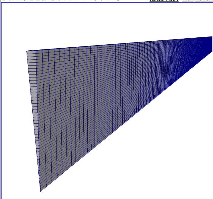
This is the inlet side Mesh which is finer as specified by the grading Factor since there are greater variations in Velocity at the inlet.
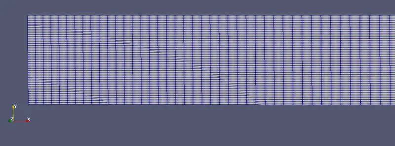
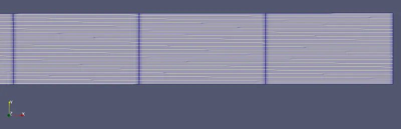
This is the Mesh at the side of outlet, the mesh is coarse as specified in the grading Factor
Results:
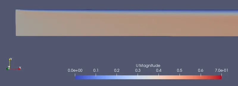
The Steady state velocity Profile at inlet
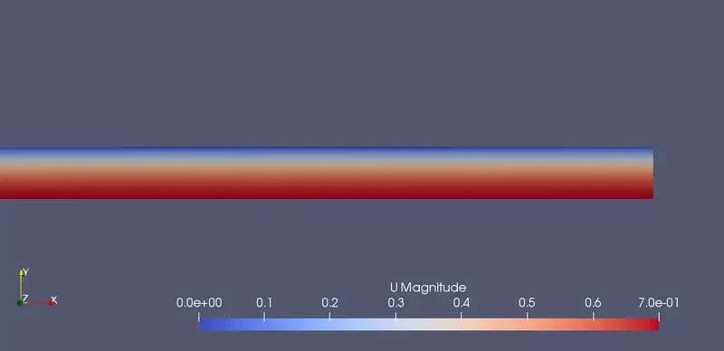
The Steady State velocity profile at outlet
The Velocity Profile along the Length of the pipe at different positions are
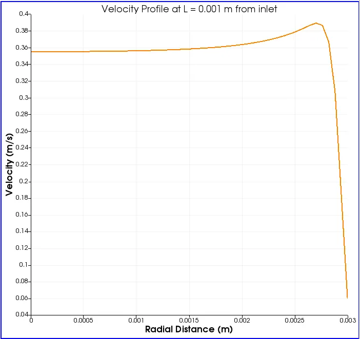
The figure below shows the Velocity variation just 0.001 from the inlet, here we can see that since we have applied the "noSlip" Boundary condition at the walls, so the velocity at walls (r = 0.003) is 0.
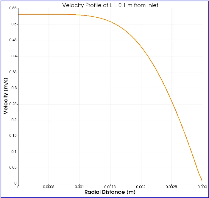
If we see the velocity profile at L = 0.1 m and L = 0.5 m from the inlet it slowly starts to develop but it's still in the Hydrodynamic Entrance Region.
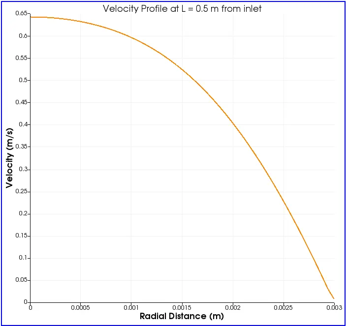
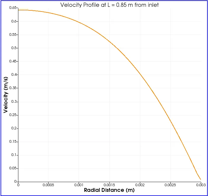
Now beyond L = 0.756 m (which is the Hydrodynamic Entrance Length(`L_e`)) the flow is completely developed and thereafter maintains the same profile.
The Pressure Variation along the Length of the pipe is given as
Further we export the data from ParaView as .csv file to compare our results with the profile obtained by solving Hagen- Poiseuille's equations.
The Matlab Code below will plot the data for all the Lengths
clear
clc
close all

%Reading the .csv File Exported from the ParaView
aa = {'L_0.001.csv','L_0.1.csv','L_0.5.csv','L_0.85.csv'};
tit = {'L = 0.001m','L = 0.1 m'...
    ,'L = 0.5 m','L = 0.85 m'};

for hh = 1:4
    f1 = fopen(aa{hh},'r');
    tline = fgetl(f1);
    n = 1;
    while 1
        tline = fgetl(f1);
        if ~ischar(tline)
            break
        end
        %disp(tline)
        l = 1;
        h = 1;
        for j = 1:length(tline)
            if(tline(j)==',')
                a(n,l) = str2double(tline(h:j-1));
                l = l+1;
                h = j+1;
            end

        end
        n = n+1;
    end
    fclose(f1);
    subplot(2,2,hh);
    U =[a(:,1);flip(a(:,1))];
    r = [a(:,6);-flip(a(:,6))];
    plot(U,r,'b','Linewidth',1.2);
    grid minor
    xlabel('Velocity(m/s)');
    ylabel('Radius(m)');
    title(tit{hh});
end

% Validating the Pressure Drop across the Length
%Reading the .csv File Exported from the ParaView
f1 = fopen('P_0.85.csv','r');
tline = fgetl(f1);
n = 1;
while 1
    tline = fgetl(f1);
    if ~ischar(tline)
        break
    end
    %disp(tline)
    l = 1;
    h = 1;
    for j = 1:length(tline)
        if(tline(j)==',')
            a(n,l) = str2double(tline(h:j-1));
            l = l+1;
            h = j+1;
        end

    end
    n = n+1;
end
fclose(f1);
P = a(:,4);
% Since it is the Kinematic Pressure we convert it back to normal Pressure
P = (997).*P;
L = a(:,6);

DP_N = abs(P(1)-P(end));
The Output of the Following Code is :
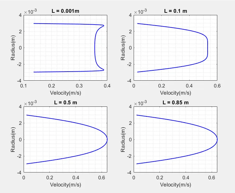
From the above figure it can be seen that how the velocity profile evolves along the length as the Flow tends to achieve a steady velocity profile
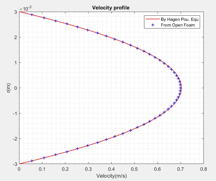
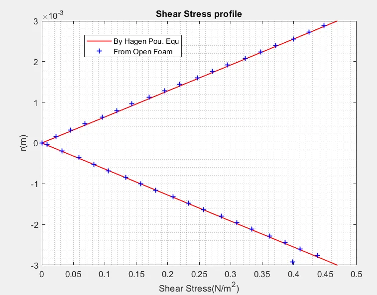
Further we also compare the Results with results from Analytical Equation (Hagen- Poiseuille's equations)
% Solving for Hagen Pousielle's Flow
clc
clear
close all

% Solving for Hagen Pousielle's Flow
% We assume a Reynold's Number of Re = 2100
Re = 2100;
% and Diameter of the Pipe is assume as
D   = 0.006;         % Diameter of Pipe in (m)
mu  = 1.0016e-3;     % Viscosity of Water (Pa.s) at 20 deg Celcius
rho = 997;           % Density of water (kg/m^3) at 20 deg Celcius
L = Re*D*0.06+0.1 ; % Length of the pipe in (m)
Ra = D/2;             % Radius of pipe

% Calculating the Average Velocity by using Re = (rho.V.D)/(mu)
Vavg = Re*mu/(rho*D);       % Average velocity
Vmax = 2*Vavg;              % Maximum Velocity
DP = 8*mu*L*Vavg/(Ra^2);     % Pressure Variation


% Velocity Profile of a fully developed laminar Flow
r = linspace(Ra,0,100);
u = 2.*Vavg.*(1-(r.^2)./(Ra.^2));
u = [u,flip(u)];
r = [r,-flip(r)];
figure(1)
plot(u,r,'r','Linewidth',1.1);
hold on
u_max = max(u);

%Reading the .csv File Exported from the ParaView
f1 = fopen('L_0.85.csv','r');
tline = fgetl(f1);
n = 1;
while 1
    tline = fgetl(f1);
    if ~ischar(tline)
        break
    end
    %disp(tline)
    l = 1;
    h = 1;
    for j = 1:length(tline)
        if(tline(j)==',')
            a(n,l) = str2double(tline(h:j-1));
            l = l+1;
            h = j+1;
        end

    end
    n = n+1;
end
fclose(f1);

U =[a(:,1);flip(a(:,1))];
R = [a(:,6);-flip(a(:,6))];
plot(U(1:3:end),R(1:3:end),'b+','Linewidth',1);
ylabel('r(m)');
xlabel('Velocity(m/s)');
title('Velocity profile ');
legend('By Hagen Pou. Equ','From Open Foam');
grid minor
U_max = max(U);

% Shear Stress profile
figure(2)
tau = sign(r).*(4.*mu.*Vavg.*r)./(Ra^2);
plot(tau,r,'r','Linewidth',1.1);
tau_wall = max(tau);
hold on
TAU = zeros(length(R),1);
% Shear Stress profile for exported data
for i = 2:length(R)
    TAU(i) = mu*((U(i-1)-U(i))./(R(i)-R(i-1)));
end
TAU = (sign(R).*TAU);
plot(TAU(1:4:end),R(1:4:end),'b+','Linewidth',1.1);
ylabel('r(m)');
xlabel('Shear Stress(N/m^2)');
title('Shear Stress profile');
legend('By Hagen Pou. Equ','From Open Foam');
grid minor
TAU_wall = max(TAU);

U_max
u_max
tau_wall
TAU_wall
The Results of the above MATLAB Code is given as
The Result Obtained from the Above Analysis can be tabulated as follows
| Max Velocity(`u_max` in `m/s`) | Wall Shear Stress (`tau_max` in `N/m^2`) | Pressure drop (`DeltaP` in `N/m^2`) | |
| By Analytical Eq | 0.7032 | 0.4696 | 267.96 |
| Numerical Analysis | 0.6895 | 0.4872 | 344.21 |
From the above comparison it is evident that the results obtained from the Numerical Computation best resembles the Analytical Equations with minimum Error