Project 1- Creating your own openFOAM solver
Aim: Modifying a existing solver to solve a scalar transport Equation for a scalar quantity "s".
Summary:
We modify the icoFoam solver which originally solves the Equation for transient incompressible flow using PISO algorithm, a pressure-velocity coupling algorithm to give us the variation of Pressure and Velocity in the Fluid Domain with time.
We have to add a scalar quantity "s" and solve a scalar transport equation for it and find out how does the variation in "s" takes place over the time.
Procedure:
1. Copying the necessary files required for the project.
For this project we select an icoFoam solver present in $FOAM_SOLVERS/incompressible/icoFoam, we will modify this solver and then use the modified solver as our solver to run the case,
Firstly we copy the icoFoam solver from $FOAM_SOLVERS/incompressible/icoFoam to our user application directory $FOAM_USER_APP
>> cd $FOAM_SOLVERS/incompressible
>> cp -r icoFoam/ $FOAM_USER_APP/icoFoam-scalar
This will copy the icoFoam directory to our user directory, further we make changes in our copied solver, thus avoiding modification in the original OpenFoam solver present in the OpenFoam directory.
We make suitable changes in the Make/files to wmake our executable in user's bin directory
We follow the same procedure and copy a case file from $FOAM_TUTORIALS/incompressible/icoFoam/cavity/cavity to our user run directory as $FOAM_RUN/scalarCavity.
>> cp -r $FOAM_TUTORIALS/incompressible/icoFoam/cavity/cavity $FOAM_RUN/scalarCavity
Once we have prepared all the things we can proceed to modify our solver .C file
2. The General Transport Equation
Now if we have a quantity "s" the general transport Equation is written as
`ubrace((dels)/(delt))_("transient terms") + ubrace(nabla.(barus))_("convective terms") = ubrace(nabla(Gammanabla.s))_("diffusive terms") + ubrace(S_s)_("Source terms")` ------------------(1)
Here `Gamma` is a Diffusivity coefficient, if we set this term to zero, than our problem will be convective, Source term in our case is 0, therefore the Equation that we solve is
`(dels)/(delt) + nabla.(barus) - nabla(Gammanabla.s) = 0`-----------------------(2)
3. Creating a dimensioned scalar as diffusivity coeff and an IOobject for scalar quantity "s" in createFields.H
Here we need to create a diffusivity coefficient as "DT" as a scalar
dimensionedScalar DT
(
    "DT",
    dimViscosity,	// Since The term will have the same dimensions as viscosity
    transportProperties

);
The value of diffusion Coefficient is given in the transportProperties present in the case
FoamFile
{
    version     2.0;
    format      ascii;
    class       dictionary;
    object      transportProperties;
}
// * * * * * * * * * * * * * * * * * * * * * * * * * * * * * * * * * * * * * //

nu              0.01;
DT              0;      // for only convective make this 0
We can also change the value of DT to control the extend of diffusion in our problem.
Further we also create an IOobject a volScalarField in createFields.H
Info<< "Reading field s\n" << endl;
volScalarField s
(
    IOobject
    (
        "s",
        runTime.timeName(),
        mesh,
        IOobject::MUST_READ,
        IOobject::AUTO_WRITE
    ),
    mesh
);
Now we have all the terms present in equation (2).
We also modify the blockMeshDict present in the case folder to suit our case.
// Here we modify the file to make a tube like mesh with one inlet, one outlet and fixed walls

FoamFile
{
    version     2.0;
    format      ascii;
    class       dictionary;
    object      blockMeshDict;
}
// * * * * * * * * * * * * * * * * * * * * * * * * * * * * * * * * * * * * * //

scale   1;

vertices
(
    (0 0 0)
    (2 0 0)
    (2 0.5 0)
    (0 0.5 0)
    (0 0 0.05)
    (2 0 0.05)
    (2 0.5 0.05)
    (0 0.5 0.05)
);

blocks
(
    hex (0 1 2 3 4 5 6 7) (100 50 1) simpleGrading (1 1 1)
);

edges
(
);

boundary
(
    inlet
    {
        type patch;
        faces
        (
            (7 3 0 4)
        );
    }

    outlet
    {
        type patch;
        faces
        (
            (2 6 5 1)
        );
    }
    fixedWalls
    {
        type wall;
        faces
        (
            (0 4 7 3)
            (2 6 5 1)
            (1 5 4 0)
	    (3 7 6 2)
        );
    }
    frontAndBack
    {
        type empty;
        faces
        (
            (0 3 2 1)
            (4 5 6 7)
        );
    }
);


// ************************************************************************* //
The Mesh can be visualised by executing following commands in case directory
>> blockMesh
>>paraFoam
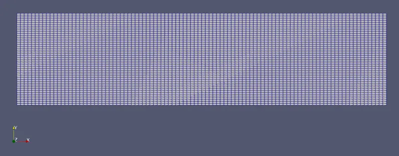
4. Creating an Initial and boundary condition for "s" in "0" folder and modifing the I.C and B.C for Velocity and Pressure.
Since we need to set a non uniform field for the scalar "s" we need to use the setFields utility by openFoam to set the Fields according to our desired way, for that we need to define "setFieldsDict" , in that we have to specify over what region in the mesh we want a particular value for "s" as our initial value.
In our case we will select a region between the inlet and oulet, and that will be close to inlet (to properly visualise), so we define 2 coordinate points that makes a box in the mesh region.
So we go into our case/system directory and create a "setFieldsDict" file.
FoamFile
{
	version 	2.0;
	format 		ascii;
	class		dictionary;
	location	"system";
	object		setFieldsDict;

}

defaultFieldValues (volScalarFieldValue s 0);

regions
(
	boxToCell
	{
		box (0.2 0 0)(0.5 0.5 0.05);
		fieldValues (volScalarFieldValue s 2);
	}

);
we also need to define a s file in our 0/ directory this is the file where the setFields utility writes all the field values
We can set it as
FoamFile
{
    version     2.0;
    format      ascii;
    arch        "LSB;label=32;scalar=64";
    class       volScalarField;
    location    "0";
    object      s;
}
// * * * * * * * * * * * * * * * * * * * * * * * * * * * * * * * * * * * * * //

dimensions      [0 0 0 0 0 0 0];

internalField   uniform 0;

boundaryField
{
    inlet
    {
        type            zeroGradient;
    }
    outlet
    {
        type            zeroGradient;
    }
    fixedWalls
    {
        type            zeroGradient;
    }
    frontAndBack
    {
        type            empty;
    }
}
once we have defined a s file in the 0/ folder we populate this s file with our custom field by executing command setFields in case directory.
>> setFields
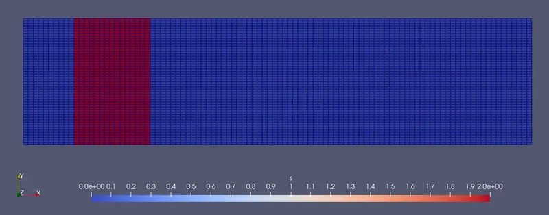
We can also visualise whether the fields are set as shown above
>> paraFoam
untick the "skip zero time step"
here we can see that we have set the value of "s" near the inlet as 2 (red color) and in other places it is 1.
5. Adding the scalar transport Equation for "s" in the solver
Now we can proceed to modify our solver "icoFoam-scalar"
We can add our scalar transport equation in the runtime while loop
// This is the Equation to Evaluate Scalar quantity s
        fvScalarMatrix sEqn(
            fvm::ddt(s)             // Transient term
            + fvm::div(phi, s)      // Convection Term
            - fvm::laplacian(DT, s) // Diffusion Term
        );
        sEqn.relax(); // applies all the relaxation factors
        sEqn.solve(); // solving the Equation
Here we use the implicit method to solve the Equation, the following Equation generates a fvScalarMatrix which is a sparse matrix, this matrix is then solved at sEqn.solve()
Further we compile the solver and store the binary in the user bin folder.
Now we can execute the solver in our case directory.
In the case directory we also need to specify the discretisation schemes for our scalar transport Equation.
fvSchemes
FoamFile
{
    version     2.0;
    format      ascii;
    class       dictionary;
    object      fvSchemes;
}
// * * * * * * * * * * * * * * * * * * * * * * * * * * * * * * * * * * * * * //

ddtSchemes
{
    default         Euler;
}

gradSchemes
{
    default         Gauss linear;
    grad(p)         Gauss linear;
}

divSchemes
{
    default         none;
    div(phi,U)      Gauss linear;
    div(phi,s)      Gauss upwind;     // here we used upwind scheme
}

laplacianSchemes
{
    default         Gauss linear orthogonal;

}

interpolationSchemes
{
    default         linear;
}

snGradSchemes
{
    default         orthogonal;
}
We also need to addin the file fvSolution
adding a "s" to the solver dictionary in fvSolution
 s
    {
	solver		smoothSolver;
	smoother	symGaussSeidel;
	tolerance	1e-05;
	relTol		0;
    }
CASE - I:
1. No Slip condition at the fixed Walls
2. Velocity at the inlet set to 4 m/s
3. Used Upwind Method for discretisation
4. DT = 0 (No Diffusion)
In this case the Intial and boundary conditions for Velocity are as follows
file 0/U
FoamFile
{
    version     2.0;
    format      ascii;
    class       volVectorField;
    object      U;
}
// * * * * * * * * * * * * * * * * * * * * * * * * * * * * * * * * * * * * * //

dimensions      [0 1 -1 0 0 0 0];

internalField   uniform (0 0 0);

boundaryField
{
    inlet
    {
        type            fixedValue;
        value           uniform (4 0 0);   // Velocity along x axis as 4 m/s
    }

    outlet
    {
        type            zeroGradient;
    }

    fixedWalls
    {
        type            noSlip;
    }

    frontAndBack
    {
        type            empty;
    }
}
Further we need to change the application in our controlDict file as
application icoFoam-scalar;
we can then execute the solver
>> icoFoam-scalar
and visualise the results as
>> paraFoam
Here we can see the variation in the scalar "s" along the direction of flow.
at t = 0 sec
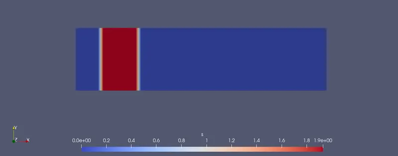
at t = 0.03 sec
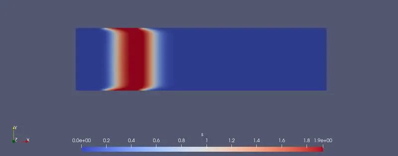
at t= 0.06 sec
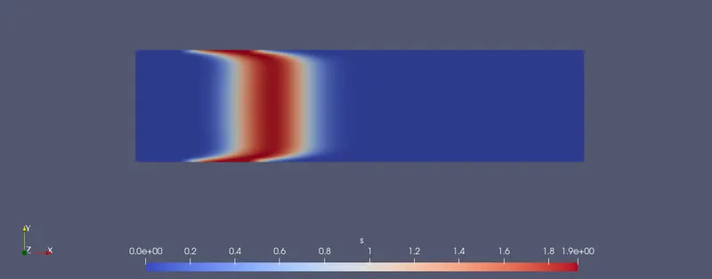
at t = 0.12 sec
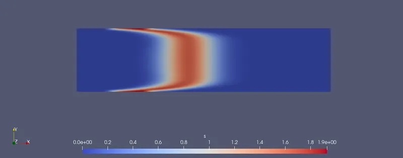
We can see that there is substantial diffusion although we set the diffusion coefficient to be zero, this is due to the lower accuracy of the upwind scheme we used in this case, and also since there was a no slip condition the scalar follows the velocity profile along the Y axis cause due to viscosity.
CASE - II:
1. Slip condition at the fixed Walls
2. Velocity at the inlet set to 4 m/s
3. Used Upwind Method for discretisation
4. DT = 0 (No Diffusion)
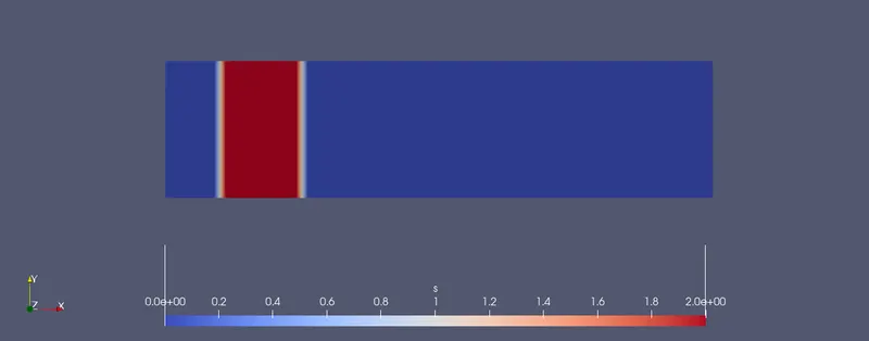
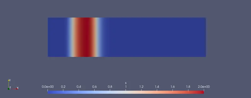
In this case we change the condition at fixed wall as slip condition,
at t= 0
at t= 0.03
at t= 0.06
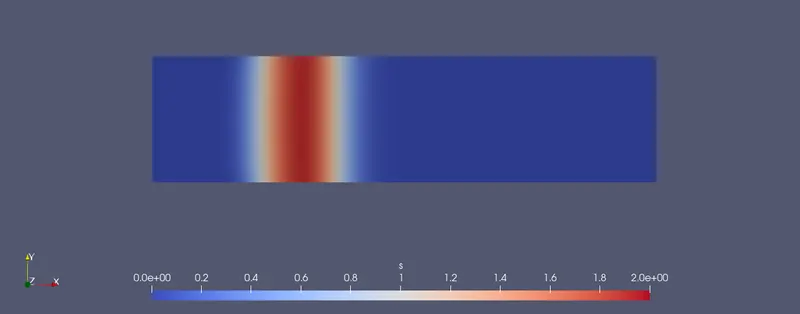
at t = 0.12
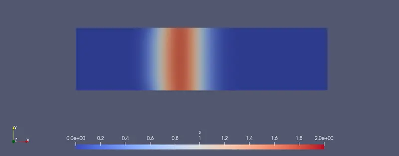
Here we can see that since we have changed the wall condition to be slip, the velocity profile is constant along Y axis, though it is a ideal flow, it helps in visualising phenomenons in a better way.
CASE - III:
1. Slip condition at the fixed Walls
2. Velocity at the inlet set to 4 m/s
3. Used van Leer TVD scheme for discretisation
4. DT = 0 (No Diffusion)
In this case we use van-Leer scheme its a TVD scheme, to use it we need to make suitable changes in our fvSchemes
as :
divSchemes
{
    default         none;
    div(phi,U)      Gauss linear;
    div(phi,s)      Gauss vanLeer;
}
Keeping all the other things as same we can proceed to solve the case
After solving we can view the results
at t = 0.03 sec
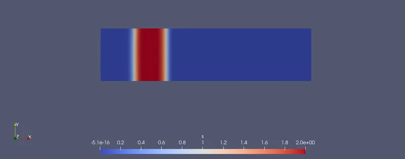
at t = 0.12 sec
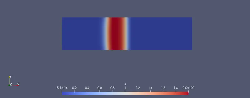
From the above image we can see that there is minumum to no numerical diffusion, since we used vanleer scheme which is a higher order scheme and also maintains its stability for abrupt changes as seen in this case.
Conclusion:
Thus we have demonstrated how the solvers can be modified to accomodate the a scalar transport Equation