Week 3.5 - Deriving 4th order approximation of a 2nd order derivative using Taylor Table method

Deriving the fourth-order approximation for second order derivative

1. Central Differencing Approximation

Now here p = 4 (Order of approximation)

and q = 2 (Order of Derivative)

The number of grid points in Central Differencing is given as p+q-1 = 4+2-1 = 5

Therefore we have to give 5 grid points in order to derive the approximation

these are (i-2),(i-1),(i),(i+1),(i+2), we have to express `f_i''(x)` in terms of `f_(i-2)(x),f_(i-1)(x),f_(i)(x),f_(i+1)(x),f_(i-2)(x)` so we assume that the approximation is in the form

`f_i''(x) ~~ (af_(i-2)(x)+bf_(i-1)(x)+cf_(i)(x)+df_(i+1)(x)+ef_(i+2)(x))/(Deltax^2)` -------(A)`

We have an approximation sign because we have neglected the trucation error which is a fourth order error.

here a,b,c,d,e are the coefficients that we have to evaluate using Taylor Table

now we consider `Deltax = h`

Expanding all the functions using Taylor Series Expansion we have

`af_(i-2)(x) =af_i(x)+a(-2h)/(1!)*f_i'(x)+a(-2h)^2/(2!)*f_i''(x)+a(-2h)^3/(3!)*f_i'''(x) +a(-2h)^4/(4!)*f_i''''(x) +...`

Doing this for all the functions `f_(i-2)(x),f_(i-1)(x),f_(i)(x),f_(i+1)(x),f_(i-2)(x)` we form the Taylor's Table

	`f_i(x)`	`f_i'(x)h`	`f_i''(x)h^2`	`f_i'''(x)h^3`	`f_i''''(x)h^4`
`a*f_(i-2)(x)`	`a`	`-2a`	`(4a)/2`	`-(8a)/6`	`(16a)/24`
`b*f_(i-1)(x)`	`b`	`-b`	`b/2`	`-b/6`	`b/24`
`c*f_(i)(x)`	`c`	`0`	`0`	`0`	`0`
`d*f_(i+1)(x)`	`d`	`d`	`d/2`	`d/6`	`d/24`
`e*f_(i+2)(x)`	`e`	`2e`	`(4e)/2`	`(8b)/6`	`(16e)/24`
Sum =	`0`	`0`	`1`	`0`	`0`

From this Taylor's Table and Equation (A) we get

`f_i''(x) h^2~~ (a+b+c+d+e)f_i(x) + (-2a-b+d+2e)f_i'(x)h+((4a)/2+b/2+0c+d/2+(4e)/2)f_i''(x)h^2+(-(8a)/6-b/6+0c+d/6+(8e)/6)f_i'''(x)h^3 +((16a)/24+b/24+0+d/24+(16e)/24)f_i''''(x)h^4`

From this Equation we get a system of Linear Equations

`a+b+c+d+e = 0` -----------(1)

`-2a-b+d+2e = 1` -----------(2)

`(4a)/2+b/2+0c+d/2+(4e)/2 = 0` -----------(3)

`-(8a)/6-b/6+0c+d/6+(8e)/6 = 0` -----------(4)

`(16a)/24+b/24+0+d/24+(16e)/24 = 0` -----------(5)

From these Equations we can solve for a,b,c,d,e

`[[1,1,1,1,1],[-2,-1,0,1,2],[4/2,1/2,0,1/2,4/2],[-8/6,-1/6,0,1/6,8/6],[16/24,1/24,0,1/24,16/24]][[a],[b],[c],[d],[e]] = [[0],[1],[0],[0],[0]]`

and its in form `A*X = B`

`X = "inv"(A)*B`

and we get the value for

`X = [[a],[b],[c],[d],[e]] = [[-1/12],[4/3],[-5/2],[4/3],[-1/12]]`

from these values of a,b,c,d,e we can form the Equation A

`f_i''(x) ~~ (-1/12f_(i-2)(x)+4/3f_(i-1)(x)-5/2f_(i)(x)+4/3f_(i+1)(x)-1/12f_(i+2)(x))/h^2`

thus we have derived the Central Difference Approximation of Fourth order

2)Skewed Right Side Difference Approximation

Now here p = 4 (Order of approximation)

and q = 2 (Order of Derivative)

The number of grid points in Central Differencing is given as p+q = 4+2 = 6

Therefore we have to give 6 grid points in order to derive the approximation

In this case we use points on the right side of the x,

these are (i),(i+1),(i+2),(i+3),(i+4),(i+5) we have to express `f_i''(x)` in terms of `f_(i)(x),f_(i+1)(x),f_(i+2)(x),f_(i+3)(x),f_(i+4)(x),f_(i+5)(x)` so we assume that the approximation is in the form

`f_i''(x) ~~ (af_(i)(x)+bf_(i+1)(x)+cf_(i+2)(x)+df_(i+3)(x)+ef_(i+4)(x)+gf_(i+5)(x))/(Deltax^2)` -------(A)`

We have an approximation sign because we have neglected the trucation error which is a fourth order error.

here a,b,c,d,e,g are the coefficients that we have to evaluate using Taylor Table

now we consider `Deltax = h`

Expanding all the functions using Taylor Series Expansion we have

Doing this for all the functions `f_(i)(x),f_(i+1)(x),f_(i+2)(x),f_(i+3)(x),f_(i+4)(x),f_(i+5)(x)` we form the Taylor's Table

	`f_i(x)`	`f_i'(x)h`	`f_i''(x)h^2`	`f_i'''(x)h^3`	`f_i''''(x)h^4`	`f_i'''''(x)h^5`
`a*f_(i)(x)`	`a`	`0`	`0`	`0`	`0`	`0`
`b*f_(i+1)(x)`	`b`	`b`	`b/2`	`b/6`	`b/24`	`b/120`
`c*f_(i+2)(x)`	`c`	`2c`	`2c`	`(4c)/3`	`(2c)/3`	`(4c)/15`
`d*f_(i+3)(x)`	`d`	`3d`	`(9d)/2`	`(9d)/2`	`(27d)/8`	`(81d)/40`
`e*f_(i+4)(x)`	`e`	`4e`	`8e`	`(32e)/3`	`(32e)/3`	`(128e)/15`
`g*f_(i+5)(x)`	`g`	`5g`	`(25e)/2`	`(125e)/6`	`(625e)/24`	`(625e)/24`
Sum =	`0`	`0`	`1`	`0`	`0`	`0`

From this Taylor's Table and Equation (A) we get

`[[1,0,0,0,0,0 ],[1,1,1/2,1/6,1/24,1/120],[1,2,2,4/3,2/3,4/15],[1,3,9/2,9/2,27/8,81/40],[1,4,8,32/3,32/3,128/15],[1,5,25/2,125/6,625/24,625/24]]*[[a],[b],[c],[d],[e],[g]] = [[0],[0],[1],[0],[0],[0]]`

and its in form `A*X = B`

`X = "inv"(A)*B`

and we get the value for

`X = [[a],[b],[c],[d],[e],[g]] = [[15/4],[-77/6],[107/6],[-13],[61/12],[-5/6]]`

from these values of a,b,c,d,e we can form the Equation A

`f_i''(x) ~~(15/4f_(i)(x)-77/4f_(i+1)(x)+107/6f_(i+2)(x)-13f_(i+3)(x)+61/12f_(i+4)(x)-5/6f_(i+5)(x))/h^2`

Thus we have derived the Skewed Right-Side Approximation Method

3)Skewed Left Side Difference Approximation

Now here p = 4 (Order of approximation)

and q = 2 (Order of Derivative)

The number of grid points in Central Differencing is given as p+q = 4+2 = 6

Therefore we have to give 6 grid points in order to derive the approximation

In this case we use points on the left side of the x,

these are (i-5),(i-4),(i-3),(i-2),(i-1),(i) we have to express `f_i''(x)` in terms of `f_(i-5)(x),f_(i-4)(x),f_(i-3)(x),f_(i-2)(x),f_(i-1)(x),f_(i)(x)` so we assume that the approximation is in the form

`f_i''(x) ~~ (af_(i-5)(x)+bf_(i-4)(x)+cf_(i-3)(x)+df_(i-2)(x)+ef_(i-1)(x)+gf_(i)(x))/(Deltax^2)` -------(A)`

We have an approximation sign because we have neglected the trucation error which is a fourth order error.

here a,b,c,d,e,g are the coefficients that we have to evaluate using Taylor Table

now we consider `Deltax = h`

Expanding all the functions using Taylor Series Expansion we have

Doing this for all the functions `f_(i-5)(x),f_(i-4)(x),f_(i-3)(x),f_(i-2)(x),f_(i-1)(x),f_(i)(x)` we form the Taylor's Table

	`f_i(x)`	`f_i'(x)h`	`f_i''(x)h^2`	`f_i'''(x)h^3`	`f_i''''(x)h^4`	`f_i'''''(x)h^5`
`a*f_(i-5)(x)`	`a`	`-5a`	`(25a)/2`	`-(125a)/6`	`(625a)/24`	`-(625a)/24`
`b*f_(i-4)(x)`	`b`	`-4b`	`8b`	`-(32b)/3`	`(32b)/3`	`-(128b)/15`
`c*f_(i-3)(x)`	`c`	`-3c`	`(9c)/2`	`-(9c)/2`	`(27c)/8`	`-(81c)/40`
`d*f_(i-2)(x)`	`d`	`-2d`	`2d`	`-(4d)/3`	`(2d)/3`	`-(4d)/15`
`e*f_(i-1)(x)`	`e`	`-e`	`e/2`	`-e/6`	`e/24`	`-e/120`
`g*f_(i)(x)`	`g`	`0`	`0`	`0`	`0`	`0`
Sum =	`0`	`0`	`1`	`0`	`0`	`0`

From this Taylor's Table and Equation (A) we get

`[[1,-5,25/2,-125/6,625/24,-625/24 ],[1,-4,8,-32/3,32/3,-128/15],[1,-3,9/2,-9/2,27/8,-81/40],[1,-2,2,-4/3,2/3,-4/15],[1,-1,1/2,-1/6,1/24,-1/120],[1,0,0,0,0,0]]*[[a],[b],[c],[d],[e],[g]] = [[0],[0],[1],[0],[0],[0]]`

and its in form `A*X = B`

`X = "inv"(A)*B`

and we get the value for

`X = [[a],[b],[c],[d],[e],[g]] = [[-5/6],[61/12],[-13],[107/6],[-77/6],[15/4]]`

from these values of a,b,c,d,e we can form the Equation A

`f_i''(x) ~~(-5/6f_(i-5)(x)+61/12f_(i-4)(x)-13f_(i-3)(x)+107/6f_(i-2)(x)-77/6f_(i-1)(x)+15/4f_(i)(x))/h^2`

Thus we have derived the Skewed Right-Side Approximation Method

Now we have also developed a MATLAB code to evaluate the taylor table coefficients for Central Difference and Skewed Methods

We have to specify the order of accuracy and the order of Derivative and the Program Evaluates the Taylor Table Matrix and also the Taylor Coefficient Matrix from inversion of Taylor's Matrix

% Deriving a Numerical Scheme using Taylor's Table 
close all
clear all
clc

% Defining the order of Approximation 
p = 4;

% Defining the order of Derivative 
q = 2;

% For Central Difference
% Number of grid points for central differencing approximation
n = p + q - 1;
%Defining the N vector for the grid points
for i = 1:n
    N_1(i) = (i-(n-(n-1)/2));
end

%For Skewed Method  
% Number of grid points for Skewed Right-side approximation
n = p + q ;
%Defining the N vector for the grid points
for i = 1:n
    N_2(i) = (i-1);
end

% Number of grid points for Skewed Left-side approximation
n = p + q ;
%Defining the N vector for the grid points
for i = 1:n
    N_3(i) = (i-(n));
end


% Deriving the Taylor's Table 
% Define the Taylor Table Matrix 
% Deriving the coefficient matrix obtained from taylor's table 
% for each individual scheme 
% k = type of Scheme
% Suffix 
% 1 = Central Differencing Approximation
% 2 = Skewed Right Side Approximation
% 3 = Skewed Left Side Approximation 

for k = 1:3
    eval(strcat("n = N_",num2str(k),"(:);"));   %Defining the type of approximation
    l = length(n);
    A = zeros(l,l);
    B = zeros(l,1);
    for i = 1:l
        for j = 1:l
            dx = n(i);
            A(i,j) = (dx^(j-1))/(factorial(j-1));
        end
    end
    A
    B(q+1,1)=1;
    % the coefficient matrix as evaluated by solving the linear system 
    eval(strcat("C_",num2str(k)," = A'\B;"));
end

% The Coefficient matrix is further used to build the numerical scheme  

% The Function Specified in the Question if f = exp(x)*cos(x) 
% Evaluating Function 
f = @(x)(exp(x)*cos(x));

% Exact Second Derivative of f 
fpp = @(x)(2*exp(x)*(-sin(x)));

% Let's Say that we calculate all the schemes for function f 
% at x = 2.5 
x = pi/3;
dx =linspace(pi/4,pi/4000,500);
error = zeros(length(dx),3);
for i = 1:length(dx)
    % By Central Differenting Method we have 
    for g = 1:length(N_1)
        f_vector(g) = f(x+N_1(g)*dx(i));
    end
    % Storing the error between approximation and exact value fpp(x) 
    error(i,1)= abs(diff([fpp(x),(f_vector*C_1)/(dx(i)^2)]));
    clear f_vector

    % By Skewed Right-side Method we have 
    for g = 1:length(N_2)
        f_vector(g) = f(x+N_2(g)*dx(i));
    end
    % Storing the error between approximation and exact value fpp(x) 
    error(i,2)= abs(diff([fpp(x),(f_vector*C_2)/(dx(i)^2)]));
    clear f_vector

    % By Skewed Right-side Method we have 
    for g = 1:length(N_3)
        f_vector(g) = f(x+N_3(g)*dx(i));
    end
    % Storing the error between approximation and exact value fpp(x) 
    error(i,3)= abs(diff([fpp(x),(f_vector*C_3)/(dx(i)^2)]));
    clear f_vector

end

loglog(dx,error(:,1),'r','linewidth',1.2);
hold on 
loglog(dx,error(:,2),'b','linewidth',1.2);
hold on 
loglog(dx,error(:,3),'k','linewidth',1.2);
hold on 
xlabel('Step Size (dx)','Interpreter','latex','FontSize',15);
ylabel('Error','Interpreter','latex','FontSize',15);
title('Log log plot of error vs Step size','Interpreter','latex','FontSize',15);
legend('Central Differencing','Skewed Right side','Skewed Left Side','Interpreter','latex','FontSize',14,'Location','best');
grid on 

This code Directly compares the result for approximations for x = pi/3 with the actual value of derivative and plots the error on log-log scale

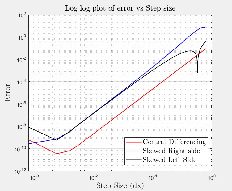
From this plot we conclude that the error is minimum for the Central Difference method, but a interesting behaviour is seen as Step size decreases, the error starts to increase again

This happens because at very low values of step size the round off errors dominate the truncation errors.

The errors in case of Skewed method are more as compared to the central Differencing, but still in some cases the Skewed methods are prefered because for central differencing we require the value from nodes on both sides to calculate the approximation

but in case of Skewed method we only require the value from nodes on either of the sides, i.e right side in case of Skewed Right-side approximation and left side in case of Skewed Left-side approximation.

For eg. in case of Time marching problems a Skewed-Left side approximation can be useful, since it requires value at node of previous time step.